Applying Under-Sampling Methods to Highly Imbalanced Data

Class imbalance can lead to a significant bias toward the dominant class, lowering classification performance and increasing the frequency of false negatives. How can we solve the problem? The most popular strategies include data resampling, which involves either undersampling the majority of the class, oversampling the minority class, or a combination of the two. As a consequence, classification performance will improve. In this article, I will describe what unbalanced data is, why Receiver Operating Characteristic Curve (ROC) fails to measure accurately, and how to address the problem. The second article, Applying Over-Sampling Methods to Highly Imbalanced Data is strongly recommended after or even before this article. The Python code in both posts for anyone who is interested is available in my github. 

What exactly is imbalanced data?

The definition of unbalanced data is simple. A dataset is considered unbalanced if at least one of the classes represents a relatively tiny minority. In finance, insurance, engineering, and many other areas, unbalanced data is common. In fraud detection, it is normal for the imbalance to be on the order of 100 to 1.

Why can’t a ROC curve measure well?

The Receiver operating characteristic (ROC) curve is a common tool for evaluating the performance of machine learning algorithms, however it does not operate well when dealing with unbalanced data. Take an insurance company as an example, which must determine if a claim is legitimate or not. The company must anticipate and avoid potentially fraudulent claims. Assume that 2% of 10,000 claims are fraudulent. The data scientist earns 98% accuracy on the ROC curve if he or she predicts that ALL claims are not fraudulent. However, the data scientist completely overlooked the 2% of actual fraudulent claims.

Let’s frame this decision challenge with either positive or negative labels. A model’s performance can be expressed by a confusion matrix with four categories. False positives (FP) are negative instances that are wrongly categorised as positives. True positives (TP) are positive examples that are appropriately identified as positives. Similarly, true negatives (TN) are negatives that are appropriately identified as negative, whereas false negatives (FN) are positive instances that are wrongly categorised as negative.

We can then define the metrics using the confusion matrix:

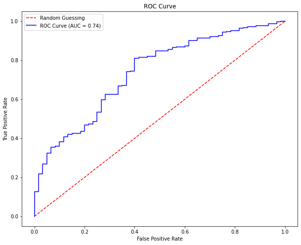
The preceding table illustrates that TPR equals TP / P, which only depends on the positive instances. The Receiver Operating Characteristic curve, as illustrated below, plots the TPR against the FPR. The AUC (Area under the curve) measures the overall classification performance. Because AUC does not prioritise one class above another, it does not adequately represent the minority class. Remember that the red dashed line in the figure represents the outcome when there is no model and the data is picked at random. The ROC curve is shown in blue. If the ROC curve is above the red dashed line, the AUC is 0.5 (half of the square area), indicating that the model outcome is no different from a fully random draw.

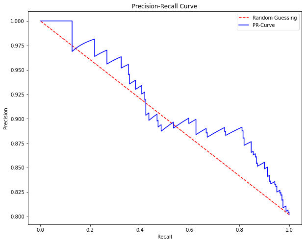
In this research, Davis and Goadrich argue that when dealing with severely imbalanced datasets, Precision-Recall (PR) curves will be more useful than ROC curves. Precision vs. recall is plotted on the PR curves. Because Precision is directly impacted by class imbalance, Precision-recall curves are more effective at highlighting differences across models in highly unbalanced data sets. When comparing various models with unbalanced parameters, the Precision-Recall curve will be more sensitive than the ROC curve.

F1 Score

The F1 score should be noted here. It is defined as the harmonic mean of precision and recall as follows:

What are the possible solutions?

In general, there are three techniques to dealing with unbalanced data: data sampling, algorithm tweaks, and cost-sensitive learning. This article will focus on data sampling procedures (others maybe in the future).

Undersampling Methods

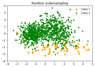
1. Random Undersampling of the majority class

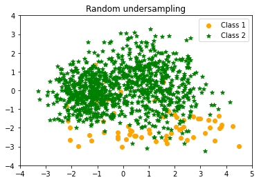
A basic under-sampling strategy is to randomly and evenly under-sample the majority class. This has the potential to result in information loss. However, if the examples of the majority class are close to one another, this strategy may produce decent results.

2. Condensed Nearest Neighbor Rule (CNN)

Some heuristic undersampling strategies have been developed to eliminate duplicate instances that should not impair the classification accuracy of the training set in order to prevent losing potentially relevant data. The Condensed Nearest Neighbor Rule (CNN) was proposed by Hart (1968). Hart begins with two empty datasets A and B. The first sample is first placed in dataset A, while the remaining samples are placed in dataset B. Then, using dataset A as the training set, one instance from dataset B is scanned. If a point in B is incorrectly classified, it is moved to A. This process is repeated until there are no points transferred from B to A.

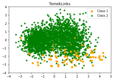
3. TomekLinks

Similarly, Tomek (1976) presented an effective strategy for considering samples around the boundary. Given two instances $a$ and $b$ that belong to distinct classes and are separated by a distance $d(a,b)$, the pair $(a, b)$ is termed a Tomek link if there is no instance $c$ such that $d(a,c) < d(a,b)$ or $d(b,c) < d(a,b)$. Tomek link instances are either borderline or noisy, thus both are eliminated.

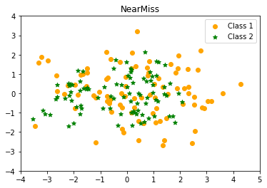
4. NearMiss

The “near neighbour” strategy and its modifications have been developed to address the issue of potential information loss. The near neighbour family’s main algorithms are as follows: first, the approach calculates the distances between all instances of the majority class and the instances of the minority class. Then, $k$ examples from the majority class with the shortest distances to those from the minority class are chosen. If the minority class has $n$ instances, the “nearest” method will return $k*n$ instances of the majority class.

“NearMiss-1” picks samples from the majority class whose average distances to the three nearest minority class instances are the shortest. “NearMiss-2” employs three of the minority class’s most remote samples. “NearMiss-3” chooses a predetermined number of closest samples from the majority class for each sample from the minority class.

5. Edited Nearest Neighbor Rule (ENN)

Wilson (1972) proposed the Edited Nearest Neighbor Rule (ENN), which requires the removal of any instance whose class label differs from at least two of its three nearest neighbours. The objective behind this strategy is to eliminate examples from the majority class that are near or close to the boundary of distinct classes based on the notion of nearest neighbour (NN) in order to improve the classification accuracy of minority instances rather than majority instances.

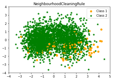
6. NeighbourhoodCleaningRule

When sampling the data sets, the neighbourhood Cleaning Rule (NCL) treats the majority and minority samples independently. NCL use ENN to eliminate the vast majority of instances. It discovers three nearest neighbours for each instance in the training set. If the instance belongs to the majority class and the classification provided by the instance’s three nearest neighbours is the opposite of the class of the chosen instance, the instance is deleted. If the chosen instance belongs to the minority class and is misclassified by its three nearest neighbours, the majority class nearest neighbours are eliminated.

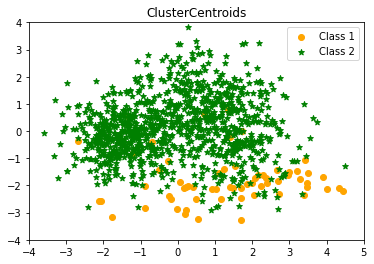
7. ClusterCentroids

This strategy undersamples the majority class by substituting a cluster of majority samples. Using K-mean techniques, this method discovers the majority class’s clusters. The cluster centroids of the N clusters are then kept as the new majority samples.

Application with Python

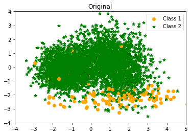
The sample strategies are demonstrated below using the python package imbalanced-learn from scikit-learn. The data generation progress (DGP) below creates 2,000 samples with two classes. The data is severely imbalanced, with 0.03 and 0.97 allocated to each class. There are ten features, two of which are informative, two of which are redundant, and six of which are repeated. The make_classification function creates the six repeated (useless) features from the informative and redundant features. The redundant features are simple linear combinations of the informative features. Each class was made up of two gaussian clusters. Informative features are drawn individually from $\mathcal{N}(0, 1)$ for each cluster and then linearly blended within each cluster. It is critical to understand that if the weights parameter is left blank, the classes are balanced.

 1
 2
 3
 4
 5
 6
 7
 8
 9
10
11
12
13
14
15
16
17
18

import pandas as pd
import numpy as np
import matplotlib.pyplot as plt
from collections import Counter
from sklearn import datasets
from sklearn.decomposition import PCA
from sklearn.model_selection import train_test_split
from sklearn.metrics import roc_curve,roc_auc_score, precision_recall_curve
from xgboost import XGBClassifier
from imblearn.datasets import make_imbalance
from imblearn.under_sampling import (RandomUnderSampler, ClusterCentroids, TomekLinks, 
                                     NeighbourhoodCleaningRule,NearMiss)

X, y = datasets.make_classification(n_samples = 4000,  n_classes = 2, n_clusters_per_class = 2, weights = [0.03,0.97], 
                                    n_features = 10, n_informative = 2, n_redundant = 2, random_state = 42)
X_train, X_test, y_train, y_test = train_test_split(X, y, test_size=0.33, random_state=42)
print(f'Original class distribution {Counter(y)}')
print(f'Training class distribution {Counter(y_train)}')

Original class distribution Counter({1: 3864, 0: 136})
Training class distribution Counter({1: 2589, 0: 91})

I use principal component analysis to reduce the dimensions and select the first two principal components for ease of visualisation. The dataset’s scatterplot is displayed below.

 1
 2
 3
 4
 5
 6
 7
 8
 9
10
11
12
13
14
15
16
17
18
19

def plot_data(X,y,method):
    
    # Use principal component to condense the 10 features to 2 features
    pca = PCA(n_components=2).fit(X)
    pca_2d = pca.transform(X)
    
    # Assign colors
    for i in range(0, pca_2d.shape[0]):
        if y[i] == 0:
            c1 = plt.scatter(pca_2d[i,0],pca_2d[i,1], c='orange', marker='o')
        elif y[i] == 1:
            c2 = plt.scatter(pca_2d[i,0],pca_2d[i,1], c='g', marker='*')  
    
    plt.legend([c1, c2], ['Class 1', 'Class 2'])
    plt.title(method)
    plt.axis([-4, 5, -4, 4]) 
    plt.show()
    
plot_data(X,y,'Original')

1
2
3
4

X_rs, y_rs = make_imbalance(X, y, sampling_strategy={1: 1000, 0: 65},
                      random_state=0)
print(f'Random undersampling {Counter(y_rs)}')
plot_data(X_rs,y_rs,'Random undersampling')

Random undersampling Counter({1: 1000, 0: 65})

 1
 2
 3
 4
 5
 6
 7
 8
 9
10
11
12
13
14
15
16
17
18
19
20
21
22
23
24
25
26
27
28
29

# RandomUnderSampler
sampler = RandomUnderSampler(sampling_strategy={1: 1000, 0: 65})
X_rs, y_rs = sampler.fit_resample(X_train, y_train)
print(f'Random undersampling {Counter(y_rs)}')
plot_data(X_rs,y_rs,'Random undersampling')

# ClusterCentroids
sampler = ClusterCentroids(sampling_strategy={1: 1000, 0: 65})
X_rs, y_rs = sampler.fit_resample(X_train, y_train)
print(f'Cluster centriods undersampling {Counter(y_rs)}')
plot_data(X_rs,y_rs,'ClusterCentroids')

# TomekLinks
sampler = TomekLinks() 
X_rs, y_rs = sampler.fit_resample(X_train, y_train)
print(f'TomekLinks undersampling {Counter(y_rs)}')
plot_data(X_rs,y_rs,'TomekLinks')

# NeighbourhoodCleaningRule
sampler = NeighbourhoodCleaningRule() 
X_rs, y_rs = sampler.fit_resample(X_train, y_train)
print(f'NearestNeighbours Clearning Rule undersampling {Counter(y_rs)}')
plot_data(X_rs,y_rs,'NeighbourhoodCleaningRule')

# NearMiss
sampler = NearMiss() 
X_rs, y_rs = sampler.fit_resample(X_train, y_train)
print(f'NearMiss{Counter(y_rs)}')
plot_data(X_rs,y_rs,'NearMiss')

Random undersampling Counter({1: 1000, 0: 65})

Cluster centriods undersampling Counter({1: 1000, 0: 65})

TomekLinks undersampling Counter({1: 2575, 0: 91})

NearestNeighbours Clearning Rule undersampling Counter({1: 2522, 0: 91})

NearMissCounter({0: 91, 1: 91})

Conclusion

I hope this post has helped you better grasp this subject. Thank you very much for reading! 😄