Linear Regression

What a better way to start my blogging journey, than with one of the most fundamental statistical learning techniques, Linear Regression. A straightforward method for supervised learning - supervised learning is the process of training a model on data where the outcome is known before applying it to data where the outcome is unknown -, learning linear regression also helps to understand the overall process of what supervised learning looks like. Linear regression, in particular, is a powerful tool for predicting a quantitative response. It's been around for a while and is the subject of a slew of textbooks. Linear Regression is part of the Generalized Linear Models family (GLM for short). Despite the fact that it may appear tedious in comparison to some of the more current statistical learning approaches, linear regression remains an effective and extensively used statistical learning method. It also provides as a useful starting point for emerging approaches. Many fancy statistical learning methods can be thought of as extensions or generalizations of linear regression. As a result, the necessity of mastering linear regression before moving on to more advanced learning approaches cannot be emphasized.
The response to the question "Is the variable $X$ associated with a variable $Y$, and if so, what is the relationship, and can we use it to predict Y?" is perhaps the most prevalent goal in statistics and linear regression tries to answer that, it does this based on linear relationships between the independent ($X$) and dependent ($Y$) variables. Simple linear regression creates a model of the relationship between the magnitudes of two variables—for example, as X increases, Y increases as well. Alternatively, when X increases, Y decreases. I've used the term simple here because we are only talking about one variable X, but instead of one variable X, we can of course use multiple predictor variables $ X_{1}...X_{n} $, which is often termed Multiple Linear Regression or just simply Linear Regression.
I assure you that I have a multitude of examples and explanations that go through all of the finer points of linear regression. But first, let's go through the fundamental concepts.
The fundamental concepts behind linear regression
-
The first step in linear regression is to fit a line to the data using least squares
-
The second step is to compute R2
-
Finally, compute the p-value for the computed R squared in the previous step
The first concept we are going to tackle is fitting a line to the data, what exactly does that mean and how can we do it? To effectively explain that we are going to need some data. I will be using the fish market data from Kaggle which is available here. The dataset contains sales records for seven common fish species seen in fish markets. Some of the features (columns) in dataset are: Species, Weight, Different Lengths, Height and Width. We’ll be using it to estimate the weight of the fish, as we are trying to explain linear regression we’ll first use only one feature to predict the weight, the height (simple linear regression)
We’ll first load the dataset using pandas read_csv:
|
|
All code in this article can be found in my Github in this repository
Now back to our first concept, fitting a line to the data, what does that mean?
Fitting a line to the data
To clearly explain this concept let’s first get only one species of fish, in this example we’ll use Perch:
|
|
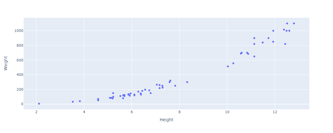
We’ll then simply create a scatter plot of Weight vs. Height.
|
|
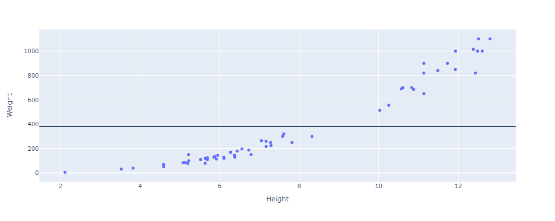
And then we’ll plot a horizontal line across the data, at the average weight (our target variable).
|
|
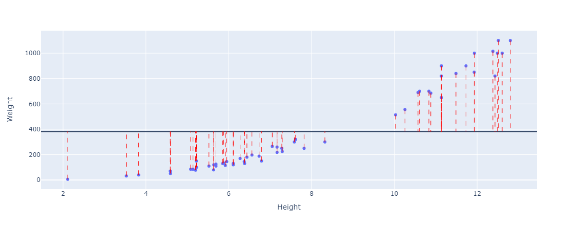
Then we calculate the difference between the actual values, the dots representing the weights in the figure, and the line (the mean value). This can be thought of as the distance between them (if you would like to think geometrically). These distances are also called the residuals. Here are the residuals plotted.
|
|
 Then we'll square each distance (residual) from the line to the data and sum them all up. We square the residuals so that the negative and positive residuals don't cancel each other out.
|
|
We get a value of 6646094.253571428. That’s a very large number, but we don’t want that we want it to be as low as possible, and how can we do that? That’s the next step.
Third we rotate and/or shift the line a little bit to be able to decrease this sum of squared distances or residuals to its lowest possible value, that is where the name least squares (or ordinary least squares) comes from. To do that we need to understand what exactly a line is mathematically.
You probably remember from linear algebra that a line is just this equation $ y = mx +b $, where $m$ is the slope of the line $b$ is the y-intercept, $x$ is the x-axis value and $y$ is the y-axis value. Well to rotate the line we need to iteratively - or mathematically - adjust the y-intercept ($b$) and the slope ($m$) so that the sum of the squared residuals - the error - is the lowest. In linear regression the equation is usually expressed in a different way like so: $\hat{y} = {\alpha} + {\beta}x$, where $ {\alpha} $ is the y-intercept (sometimes also written as $ {\beta}_0 $) and $ {\beta} $ is the slope. In simple linear regression there is only one independent variable - feature - and therefore only one slope - or coefficient -, but in many cases we have many different features that we would like to use in our equation so for every feature $X_n$ added we add its coefficient $ {\beta}_n$, to be estimated with the y-intercept. In general, such a relationship may not hold perfectly for the mostly unobserved population of values of the feature and target variables; these unobserved variations from the above equation are referred to as random errors or noise, which we assume on average is zero, so during modelling of the linear regression line it is omitted from the parameters to estimate. And they are usually added to the equation as well to get: $\hat{y} = {\alpha} + {\beta}x + {\epsilon}_i$.
But now comes the real question how does linear regression adjust the y-intercept and coefficients to get the “best-fitting” line which yields the lowest sum of squared residuals. Recall that I mentioned that these parameters ($\hat{\alpha}$ and $\hat{\beta}$) can be either estimated iteratively or mathematically. In the third step I mentioned that we rotate the line a little bit to be able to decrease the sum of squared residuals, well that is actually the iterative approach, which is conducted using an optimization technique named gradient descent. The mathematical approach uses derived equations using calculus to estimate these parameters, analytically straight away to get the line. In this article I’ll talk about these equations i.e. the mathematical approach, and will leave the iterative approach using gradient descent for another article where I talk about gradient descent in general as it is widely used in many other machine learning algorithms (not only linear regression) to minimize a loss or cost function (or gradient ascent to maximize an objective function) and it does that by iteratively adjusting these parameter, in linear regression the sum of squared residuals is the loss function.
First let’s define the sum of squared residuals equations, we know that the equation for the line is: $ \hat{y} = {\alpha} + {\beta}x$, and we know that the residuals is the actual value $y$ minus the estimated value (which we will give the symbol $\hat{y}$), the result is then squared. So the sum of squared residuals is defined by:
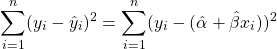
where $n$ is the sample size.
we can shorten this to a function with $ \hat{\alpha} $ and $ \hat{\beta} $ as parameters, $ F(\hat{\alpha},\hat{\beta}) $. To minimize this equation, we use calculus, which is great in such problems (if the function is differentiable).
How does it do that?
- It takes the partial derivatives of the function ($ F(\hat{\alpha},\hat{\beta}) $) with respect to $ \hat{\alpha} $ and $ \hat{\beta} $
- Sets the partial derivatives equal to 0
- Finally, solve for $ \hat{\alpha} $ and $ \hat{\beta} $
We could examine the second-order conditions to make sure we identified a minimum and not a maximum or a saddle point. I’m not going to do that here, but rest assured that our calculations will result in the smallest sum of squared residuals achievable. I will also not explain all the derivation steps of the partial derivatives here but simply give them. The first partial derivative with respect to $\hat{\alpha}$ is: $\frac {\partial} {\partial\hat{\alpha}} = -2 \sum_{i=1}^{n} (y_i - (\hat{\alpha} + {\hat{\beta}}x_i)) $
and the second partial derivative with respect to $\hat{\beta}$ is: $\frac {\partial} {\partial\hat{\beta}} = -2 \sum_{i=1}^{n} x_i(y_i - (\hat{\alpha} + {\hat{\beta}}x_i)) $
Now we set these partial derivatives equal to zero:
For $\hat{\alpha}$ : $ -2 \sum_{i=1}^{n} (y_i - (\hat{\alpha} + {\hat{\beta}}x_i)) = 0 $ (1)
For $\hat{\beta} $ : $ -2 \sum_{i=1}^{n} x_i(y_i - (\hat{\alpha} + {\hat{\beta}}x_i)) = 0 $ (2)
Now we have 2 equations and 2 unknowns, and we are going to solve these to find our optimal parameters, how do we do that? First we get an expression for $ \hat{\alpha} $ that solves for it using the first equation and, which we will then substitute in the second equation to solve for $ \hat{\beta} $.
The first expression that solves for $\hat{\alpha}$ ends up to be: $ \hat{\alpha} = \bar{y} - \hat{\beta}\bar{x} $, where $\bar{y}$ and $\bar{x}$ are the averages of both variables. When we substitute this expression for the partial derivative equation for $ \hat{\beta} $ we get: $\frac {\sum_{i=1}^{n} (x_i - \bar{x})(y_i - \bar{y})}{\sum_{i=1}^{n} (x_i-\bar{x})^2} $
With these equations in hand we can easily estimate the parameters and fit a line to the data that will give us the minimum sum of squared residuals. Let’s implement that in python:
|
|
We can then use this function for our data to get the best fitting line:
|
|
The least squares function determines that the best values for the parameters, $\hat{\alpha}$ and $\hat{\beta}$ that minimize the sum of squared residuals are: -537.3275192931233 and 116.96540985551397 respectively.
We can also visualize that using plotly (my favourite plotting library 😊):
|
|
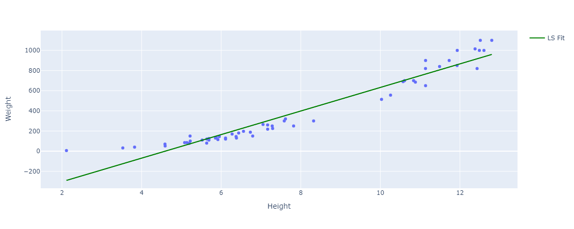
We can compare these estimated/learned parameters with scikit-learns LinearRegression solution as well:
|
|
Intercept: -537.3275192931234 Coefficient: 116.96540985551398
They are similar as scikit-learns LinearRegression also uses scipys linalg.lstsq, which computes the least squares solution.
We can also visualize the residuals with respect to this line:
|
|
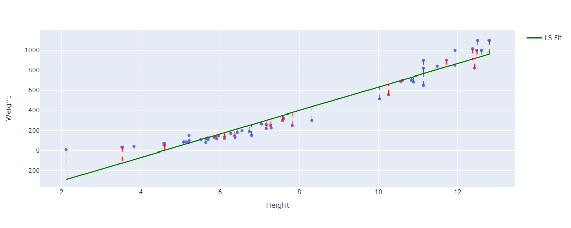
We can see they are very small residuals which is exactly what we want. We can also quantify the residuals, using our sum of squared residuals to get the lowest possible value which in this case is: 412872.84783624834 which is a great improvement from 6646094.253571428, but linear regression is usually evaluated using the mean squared error. The mean squared error is just the sum of squared residuals divided by $ n $, the sample size. Which in this simple case is 56, that gives us a mean squared error of: 7372.7294256472915.
|
|
412872.84783624834
7372.7294256472915.
or by using scikit-learns mean_squared_error in the metrics module
|
|
7372.7294256472915.
Other evaluation metrics such as mean absolute error, root mean squared error and R2 are used for linear regression as well. Which brings us to our second concept calculating R2.
Computing R2 or Coefficient of Determination
This metric represents the proportion of the dependent variable’s variation explained by the model’s independent variables. It assesses the adequacy of your model’s relationship with the dependent variable. Consider the following scenario in which we estimate the error of the model with and without knowledge of the independent variables to better grasp what R2 really means.
When we know the values of the independent variable ($X$), we can calculate the sum of squared residuals (SSR for short) as discussed above. Which we know is the difference between the actual value and the value on the line (predicted value) squared, summed over all data points. And with consider the situation where the independent variable’s values are unknown and only the $y$ values are available. The mean of the $y$ values is then calculated, then the mean can be represented by a horizontal line, as seen above, we now calculate the sum of squared residuals between the mean $y$ value and all other $y$ values. This sum of squared residuals between the mean $y$ value and all other $y$ values is termed as the total sum of squares (TSS for short), which is the total variation in $y$. Why the mean? Because the mean is the simplest model we can fit and hence serves as the model to which the least squares regression line is compared to.
$$ TSS = \sum_{i=1}^{n} (y_i - \bar{y}) ^ 2 $$
As a result, we’d like to know what proportion of the total variation of $y$ is explained by the independent variable $x$. We may derive the coefficient of determination or R2 by subtracting the proportion of the total variation of $y$ that is not represented by the regression line from 1, to get:
$$ R^2 = 1 - \frac {SSR}{TSS} $$
which represents that part of the variance of $y$ that is described by the independent variable $x$. In our case we can calculate it like so:
|
|
0.9378773709665068
or by using scikit-learns r2_score
|
|
0.9378773709665068
The sum of squared residuals (SSR) to total sum of squares (TSS) ratio indicates how much overall error is left in your regression model. By subtracting that ratio from one, you can calculate how much error you were able to eliminate using regression analysis. This is R2. If R2 is high (it’s between 0 and 1), the model accurately depicts the dependent variable’s variance. If R2 is very low, the model does not represent the dependent variable’s variance, and regression is no better than taking the mean value, i.e. no information from the other variables is used. A negative R2 indicates that you are performing worse than the average. It can be negative if the predictors fail to explain the dependent variables at all. As a result, R2 assesses the data points that are scattered about the regression line. A model with an R2 of 1 is almost impossible to find. In that situation, all projected values are identical to actual values, implying that all values lie along the regression line or that the model is over-fitting the data, which in this case might require some regularisation (Lasso or Ridge Regression), I’ll talk about these in a seperate blog post. However, don’t be fooled by the R2 value. A good model may have a low R2 value, while a biased model may have a high R2. It is for this reason that residual plots should be used:
|
|
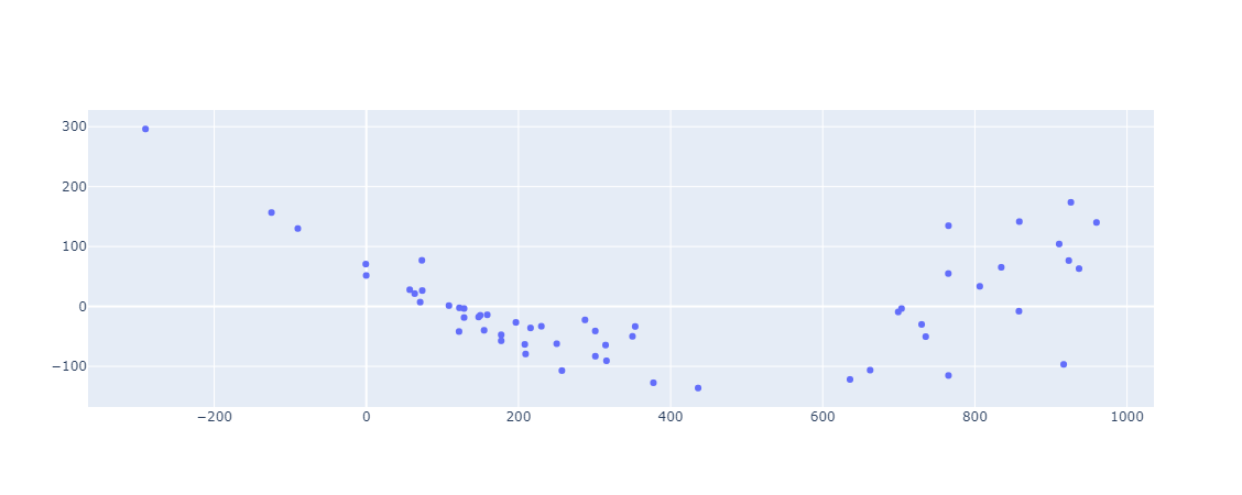
And as we can see they are randomly scattered around zero.
How significant is the R2?
We need a way to determine if the R2 value is statistically significant. We need a p-value to be more precise. The main idea behind the p-value for R2 is determined by the F-statistic. Which is a statistic that expresses how much of the model has improved (compared to the mean) given the inaccuracy of the model, which we can calculate a p-value for to get the significance of R2. The F-statistic is expressed in the following way:
$ F = \frac {(TSS- RSS)/(p-1)}{RSS/(n-p)} $
where $p$ is the number of predictors (including the constant) and $n$ is the number of observations or sample size, these are the degrees of freedom that turn the sums of squares into variances. We can interpret the nominator as the variation in fish weight explained by height and the denominator as the variation in fish weight NOT explained by fish height i.e. the variation that remains after fitting the line. If the “fit” was good then the nominator will be a large number and the denominator a small number which should yield a large F-statistic, the opposite otherwise. The question remains, where is the p-value? or more precisely how do we turn this number - F-statistic - to a p-value.
To determine the p-value, we generate a set of random data, calculate the mean and sum of squares around the mean, and then calculate the fit and sum of squares around the fit. After that, plug all of those values into the F-statistic equation to get a number. Then plot that number in a histogram, and repeat the process as many times as necessary. We return to our original data set once we’ve finished with our random data sets. The numbers are then entered into the F-statistic equation in this case. The p-value is calculated by dividing the number of more extreme values by the total number of values. Our F-statistic is:
|
|
815.2484661408347
All of this is usually done with software and we can do that in python using statsmodels OLS like so:
|
|
which results in the following table with all information including the coefficients, the intercept, R2, F-statistic and the p-value for it, which in this case is $2.9167 × 10^{-34}$ and if the p-value is less than a significance level (usually 0.05) then the model fits the data well (true in this case).
| Dep. Variable: | Weight | R-squared: | 0.938 |
|---|---|---|---|
| Model: | OLS | Adj. R-squared: | 0.937 |
| Method: | Least Squares | F-statistic: | 815.2 |
| Date: | Fri, 18 Mar 2022 | Prob (F-statistic): | 2.92e-34 |
| Time: | 14:21:40 | Log-Likelihood: | -328.82 |
| No. Observations: | 56 | AIC: | 661.6 |
| Df Residuals: | 54 | BIC: | 665.7 |
| Df Model: | 1 | ||
| Covariance Type: | nonrobust |
| coef | std err | t | P>|t| | [0.025 | 0.975] | |
|---|---|---|---|---|---|---|
| const | -537.3275 | 34.260 | -15.684 | 0.000 | -606.015 | -468.640 |
| x1 | 116.9654 | 4.096 | 28.553 | 0.000 | 108.752 | 125.178 |
| Omnibus: | 11.275 | Durbin-Watson: | 0.678 |
|---|---|---|---|
| Prob(Omnibus): | 0.004 | Jarque-Bera (JB): | 11.319 |
| Skew: | 0.954 | Prob(JB): | 0.00349 |
| Kurtosis: | 4.099 | Cond. No. | 24.8 |
These are the main and most fundamental ideas behind linear regression, but of course there are more in-depth topics regarding linear regression such as multicolinearity, categorical variables, cofounding variables, outliers, influential values, heteroskedasticity, non-normality, correlated errors, regularisation and polynomial regression. Polynomial regression is normal linear regression but just with polynomial features which are feature crosses (combinations & exponents). Polynomial features are usually computed by multiplying features together and/or raising features to a user-selected degree. Scikit-learn preprocessing module implements this using its PolynomialFeatures class that also gives you the option to keep interaction features, which are “…features that are products of at most degree distinct input features, i.e. terms with power of 2 or higher of the same input feature are excluded”. I will try my best to write about these different topics in seperate blog posts.
Thank you very much for reading all the way through, and I hope you enjoyed the article. See you in the next article and, Stay Safe!