Logistic Regression: With Application and Analysis on the 'Rain in Australia' Dataset

The logistic model (or logit model) in statistics is a statistical model that represents the probability of an event occurring by making the log-odds for the event a linear combination of one or more independent variables.

Logistic regression is another approach borrowed from statistics by machine learning. It is the go-to strategy for binary classification problems (problems with two classes) even though it is a regression algorithm (predicts probabilities, more on that later).

For example,

• To predict whether an email is spam (1) or not (0)
• Whether the tumor is malignant (1) or not (0)

This post will discuss the logistic regression algorithm for machine learning.

What’s the Problem with Linear Regression for Classification?

The linear regression model is effective for regression but ineffective for classification. Why is this the case? If you have two classes, you may label one with 0 and the other with 1 and use linear regression. It works technically, and most linear model programmes will generate weights for you. However, there are a couple issues with this approach:

• A linear model does not produce probabilities, but rather treats the classes as integers (0 and 1) and finds the optimum hyperplane (for a single feature, a line) that minimises the distances between the points and the hyperplane. As a result, it just interpolates between the points and cannot be interpreted as probabilities.
• A linear model will also extrapolate numbers below zero and above one. This is a promising hint that there may be a more intelligent method to classification.
• Linear models are not applicable to multi-class classification issues. The next class would have to be labelled with 2, then 3, and so on. Although the classes may not be in any meaningful order, the linear model would impose an odd structure on the relationship between the features and your class predictions. The higher the value of a positive-weighted feature, the more it contributes to the prediction of a class with a higher number, even if classes with similar numbers are not closer than other classes.

Because the predicted outcome is a linear interpolation between points rather than a probability, there is no meaningful threshold at which one class can be distinguished from the other. A decent example of this problem may be seen on Stackoverflow.

So what can be a solution to classification problems, well there are many but one solution is logistic regression, here come the logistic function (or the sigmoid function)

The Logistic Function

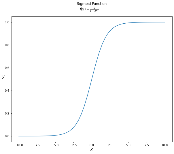
Logistic regression is named after the logistic function, which is at the heart of the algorithm. The logistic function, also known as the sigmoid function, was devised by statisticians to characterise the characteristics of rapid population expansion in ecology that exceeds the carrying capacity of the ecosystem (check here). It’s an S-shaped curve that can transfer any real-valued integer to a value between 0 and 1, but never exactly between those bounds. $$f(z) = \frac{1}{1 + e^{-z}}$$

Where $e$ is the natural logarithm base (Euler’s number) and z is the actual numerical value to be transformed.

Below we can see the logistic/sigmoid function applied to a range of numbers between -10 and 10 transformed into the range 0 and 1 using the logistic function.

Now that we’ve defined the logistic function, let’s look at how it’s employed in logistic regression.

Logistic Regression Algorithm Representation

Logistic regression, like linear regression, uses an equation as its representation. The transition from linear regression to logistic regression is rather simple. We used a linear equation to model the link between the outcome and the features in the linear regression model:

We prefer probabilities between 0 and 1 for classification, so we wrap the right side of the equation in the logistic function. This constrains the output to only accept values between 0 and 1.

To predict the output value ($y$), the input values ($X$) are linearly combined using weights or coefficient values (referred to as the Greek capital letter Beta). The coefficients in the equation are the real representation of the model that you would store in memory or in a file.

Why Logistic Regression is Regression not Classification

Simply put, logistic regression predicts probabilities which are continous values (i.e., regression).The probability of the default class is modelled using logistic regression (e.g. the first class). For example, if we are modelling people’s gender based on their height as male or female, the first class may be male, and the logistic regression model could be expressed as the probability of male given a person’s height, or more formally:

In other words, we are modelling the probability that an input (X) belongs to the default class (Y=1); we can express this formally as:

Logistic regression is a linear method, however the logistic function is used to alter the predictions. As a result, we can no longer understand the predictions as a linear combination of the inputs, as we can with linear regression. To continue from above, the model can be described as:

We can transform the previous equation as follows (remembering that we may eliminate the $e$ (exp) from one side by adding a natural logarithm ($ln$) to the other):

This is beneficial because we can see that the output on the right is linear again (exactly like linear regression), and the input on the left is a log of the likelihood of the default class. This ratio on the left is known as the default class’s odds (it’s historical that we use odds rather than probabilities; for example, odds are used in boxing rather than probabilities). Odds are calculated as a ratio of the event’s likelihood divided by the event’s probability of not occurring. For example, 0.5/(1-0.5) which has the odds of 1. So we could instead write:

Because the odds are log transformed, the left hand side is referred to as the log-odds or the probit. Although different types of functions can be used for the transform, the transform that relates the linear regression equation to the probabilities is commonly referred to as the link function, for example, the probit link function.

We can reposition the exponent to the right and write it as:

All of this helps us understand that the model is still a linear combination of the inputs, but that this linear combination is related to the default class’s log-odds.

Learning the Logistic Regression Model Parameters

The logistic regression algorithm’s coefficients must be estimated using your training data. This is typically accomplished through the use of maximum-likelihood estimation (gradient-descent can also be used, article on that in the future)

Although it does make assumptions about the distribution of your data, maximum-likelihood estimation (MLE) is a frequent learning method utilised by a variety of machine learning algorithms.

The best coefficients would result in a model that predicted a value very close to 1 (for example, male) for the default class and a value very close to 0 (for example, female) for the other class. The idea behind maximum-likelihood logistic regression is that a search algorithm seeks coefficient values that minimise the error (see The loss function) between the probabilities predicted by the model and those in the data (e.g. probability of 1 if the data is the primary class). It is sufficient to state that a minimization algorithm is utilised to optimise the coefficient values for the training data.

The loss function and MLE

So, to learn the coefficients ($\beta$) of a logistic regression model, we need to define a cost function. MLE is a specific type of probability model estimation, where the loss/objective function is the log likelihood (or minimizing the negative log likelihood) denoted by $\mathcal{L}$.

Suppose we have a set of experimental observations:

and a class of distributions $p(x;\theta)$, where $\theta$ is a set of parameters on which the form of $p$ depends. The MLE for the distribution from which the dataset has been extracted is defined as the one which maximizes the quantity

as $\theta$ varies. Therefore, in the hypothesis that variables are i.i.d. (Independent and identically distributed) the best value for $\theta$ will be given by

Because multiplication easily overflows/underflows, the equivalent expression is frequently used instead of this one

Let’s look at how this method can be used to construct the log-likelihood loss function (also known as cross-entropy).

Surprisingly, while training machine learning algorithms, the maximum likelihood estimation method can be used to create loss functions. In fact, one can imagine working in a scenario in which a dataset with specific statistical qualities is generated, and then construct a loss function that takes those properties into account automatically.

Log likelihood or cross-entropy is the mainly used loss function in classification problems, namely problems in which the underlying distribution has a discrete set of output values. Just as an example one can imagine a Bernoulli distribution, which has two outputs, one having probability $p$ and the other $(1−p)$ of being extracted. The negative log likelihood is defined as

and in information theory it quantifies the average number of bits needed to identify an event drawn from a set if a coding scheme used for the set is optimized for an estimated probability distribution $q$, rather than the true distribution $p$. This quantity can also be derived using MLE. Suppose data extracted according to a distribution $p(x)$ and an estimated distribution $q(x)$. Let’s also define the class of estimated probability distributions $\hat{y} = \hat{g}(x; \vec{\theta})$. Then the optimal parameters are obtained minimizing

where $\Omega$ is the sample space on which the probability space is defined. This way negative log likelihood is recovered as well.

Prediction with Logistic Regression

Predictions with a logistic regression model are as easy as plugging numbers into the logistic regression equation and computing the result.

Let’s put this into context with an example. Imagine that we had a model that can determine a person’s gender based on their height (completely fictitious). Is the person male or female given a height of 192cm?

Assuming we now know (learned) the coefficients $\beta_{0} = -70$ and $\beta_{1} = 0.4$. Using the aforementioned equation, we can determine the probability of a male given a height of 165cm, or $P(male|height=165)$.

Or a very low probability of that the person is a male.

In practise, the probabilities can be used immediately. Because this is a classification problem and we want a useful result, we can convert the probabilities to a binary class value, such as

Using Logistic Regression on a dataset

I’ll be using the Rain In Australia dataset found in kaggle. The dataset contains information regarding daily weather measurements from a variety of sites in Australia and the aim is to predict whether it will rain the next day or not (Yes or No), which is a binary classification problem that is well suited for logistic regression.

I implemented Logistic Regression with Python and Scikit-Learn using its LogisticRegression class. All code can be found in my github.

I first import the libraries and load the dataset.

 1
 2
 3
 4
 5
 6
 7
 8
 9
10
11
12
13

import pandas as pd
import numpy as np
import matplotlib.pyplot as plt
import seaborn as sns
from sklearn.linear_model import LogisticRegression
from sklearn.model_selection import train_test_split
from sklearn.preprocessing import MinMaxScaler
from sklearn.metrics import accuracy_score
from sklearn.metrics import confusion_matrix
from sklearn.metrics import classification_report
import category_encoders as ce

df = pd.read_csv("./data/weatherAUS.csv")

Then I conduct some Exploratory Data Analysis (EDA), some cleaning and data preparation for modelling

Dataset shape

1

df.shape

(145460, 23)

Preview the dataset

1

df.head()

Get column names

1
2

for col in df.columns.values.tolist():
    print(col+",", end=' ') 

Date, Location, MinTemp, MaxTemp, Rainfall, Evaporation, Sunshine, WindGustDir, 
WindGustSpeed, WindDir9am, WindDir3pm, WindSpeed9am, WindSpeed3pm, 
Humidity9am, Humidity3pm, Pressure9am, Pressure3pm, Cloud9am, Cloud3pm, 
Temp9am, Temp3pm, RainToday, RainTomorrow

View summary of dataset

1

df.info()

<class 'pandas.core.frame.DataFrame'>
RangeIndex: 145460 entries, 0 to 145459
Data columns (total 23 columns):
 #   Column         Non-Null Count   Dtype  
---  ------         --------------   -----  
 0   Date           145460 non-null  object 
 1   Location       145460 non-null  object 
 2   MinTemp        143975 non-null  float64
 3   MaxTemp        144199 non-null  float64
 4   Rainfall       142199 non-null  float64
 5   Evaporation    82670 non-null   float64
 6   Sunshine       75625 non-null   float64
 7   WindGustDir    135134 non-null  object 
 8   WindGustSpeed  135197 non-null  float64
 9   WindDir9am     134894 non-null  object 
 10  WindDir3pm     141232 non-null  object 
 11  WindSpeed9am   143693 non-null  float64
 12  WindSpeed3pm   142398 non-null  float64
 13  Humidity9am    142806 non-null  float64
 14  Humidity3pm    140953 non-null  float64
 15  Pressure9am    130395 non-null  float64
 16  Pressure3pm    130432 non-null  float64
 17  Cloud9am       89572 non-null   float64
 18  Cloud3pm       86102 non-null   float64
 19  Temp9am        143693 non-null  float64
 20  Temp3pm        141851 non-null  float64
 21  RainToday      142199 non-null  object 
 22  RainTomorrow   142193 non-null  object 
dtypes: float64(16), object(7)
memory usage: 25.5+ MB

• We can see that the dataset contains mixture of categorical and numerical variables.
• Categorical variables have data type object.
• Numerical variables have data type float64.
• Also, there are some missing values in the dataset. We will explore it later.

View statistical properties of dataset

1

df.describe() 

Univariate Analysis

Explore RainTomorrow target variable

1
2
3

#Check for missing values

df['RainTomorrow'].isnull().sum()

3267

1
2
3

#Drop Null values of RaiNTomorrow column

df.dropna(subset=['RainTomorrow'], inplace=True)

1
2
3
4

#Number of unique values and the values

print(df['RainTomorrow'].nunique())
print(df['RainTomorrow'].unique())

2
['No' 'Yes']

As expected only 2 values (Yes or No)

1
2
3
4
5
6

# Check the frequency distribution of the values

print(df['RainTomorrow'].value_counts())

#Or in percentage
df['RainTomorrow'].value_counts()/len(df)

No     110316
Yes     31877
Name: RainTomorrow, dtype: int64

No     0.775819
Yes    0.224181
Name: RainTomorrow, dtype: float64

We see an unbalanced problem

1
2
3
4

# Visualize frequency distribution of RainTomorrow variable
f, ax = plt.subplots(figsize=(8, 4))
ax = sns.countplot(y="RainTomorrow", data=df, palette="Set2")
plt.show()

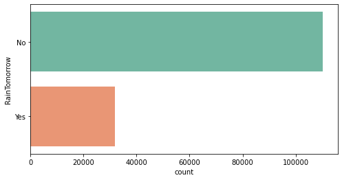
Findings of Univariate Analysis

• The number of unique values in RainTomorrow variable is 2.
• The two unique values are No and Yes.
• Out of the total number of RainTomorrow values, No appears 77.58% times and Yes appears 22.42% times.

Bivariate Analysis

Types of variables

In this section, I segregate the dataset into categorical and numerical variables. There are a mixture of categorical and numerical variables in the dataset. Categorical variables have data type object. Numerical variables have data type float64.

First of all, I will find categorical variables.

1
2
3
4

categorical = df.select_dtypes(include=['object']).columns

print('There are {} categorical variables\n'.format(len(categorical)))
print('The categorical variables are :', categorical.tolist())

There are 7 categorical variables
The categorical variables are : ['Date', 'Location', 'WindGustDir', 
'WindDir9am', 'WindDir3pm', 'RainToday', 'RainTomorrow']

1
2
3

# View the categorical variables

df[categorical].head()

Summary of categorical variables

• There is a date variable. It is denoted by Date column.
• There are 6 categorical variables. These are given by Location, WindGustDir, WindDir9am, WindDir3pm, RainToday and RainTomorrow.
• There are two binary categorical variables - RainToday and RainTomorrow.
• RainTomorrow is the target variable

Explore problems within categorical variables

First, I will explore the categorical variables.

1
2
3

# Missing values in categorical variables

df[categorical].isnull().sum()

Date                0
Location            0
WindGustDir      9330
WindDir9am      10013
WindDir3pm       3778
RainToday        1406
RainTomorrow        0
dtype: int64

1
2
3
4
5

# print categorical variables with missing values

cat_missing = [col for col in categorical if df[col].isnull().sum()!=0]

print(df[cat_missing].isnull().sum())

WindGustDir     9330
WindDir9am     10013
WindDir3pm      3778
RainToday       1406
dtype: int64

We can see that there are only 4 categorical variables in the dataset which contains missing values. These are WindGustDir, WindDir9am, WindDir3pm and RainToday

 1
 2
 3
 4
 5
 6
 7
 8
 9
10

# Frequency count of categorical variables
from IPython.display import Markdown, display
def printmd(string):
    display(Markdown(string))
    
for col in categorical: 
    if col == "Date":
        continue
    printmd(f'**{col}**')
    print(df[col].value_counts())

Location

Canberra            3418
Sydney              3337
Perth               3193
Darwin              3192
Hobart              3188
Brisbane            3161
Adelaide            3090
Bendigo             3034
Townsville          3033
AliceSprings        3031
MountGambier        3030
Launceston          3028
Ballarat            3028
Albany              3016
Albury              3011
PerthAirport        3009
MelbourneAirport    3009
Mildura             3007
SydneyAirport       3005
Nuriootpa           3002
Sale                3000
Watsonia            2999
Tuggeranong         2998
Portland            2996
Woomera             2990
Cairns              2988
Cobar               2988
Wollongong          2983
GoldCoast           2980
WaggaWagga          2976
Penrith             2964
NorfolkIsland       2964
SalmonGums          2955
Newcastle           2955
CoffsHarbour        2953
Witchcliffe         2952
Richmond            2951
Dartmoor            2943
NorahHead           2929
BadgerysCreek       2928
MountGinini         2907
Moree               2854
Walpole             2819
PearceRAAF          2762
Williamtown         2553
Melbourne           2435
Nhil                1569
Katherine           1559
Uluru               1521
Name: Location, dtype: int64

WindGustDir

W      9780
SE     9309
E      9071
N      9033
SSE    8993
S      8949
WSW    8901
SW     8797
SSW    8610
WNW    8066
NW     8003
ENE    7992
ESE    7305
NE     7060
NNW    6561
NNE    6433
Name: WindGustDir, dtype: int64

WindDir9am

N      11393
SE      9162
E       9024
SSE     8966
NW      8552
S       8493
W       8260
SW      8237
NNE     7948
NNW     7840
ENE     7735
ESE     7558
NE      7527
SSW     7448
WNW     7194
WSW     6843
Name: WindDir9am, dtype: int64

WindDir3pm

SE     10663
W       9911
S       9598
WSW     9329
SW      9182
SSE     9142
N       8667
WNW     8656
NW      8468
ESE     8382
E       8342
NE      8164
SSW     8010
NNW     7733
ENE     7724
NNE     6444
Name: WindDir3pm, dtype: int64

RainToday

No     109332
Yes     31455
Name: RainToday, dtype: int64

RainTomorrow

No     110316
Yes     31877
Name: RainTomorrow, dtype: int64

1
2
3
4

# check for cardinality in categorical variables
for col in categorical:
    
    print(col, ' contains ', len(df[col].unique()), ' labels')

Date  contains  3436  labels
Location  contains  49  labels
WindGustDir  contains  17  labels
WindDir9am  contains  17  labels
WindDir3pm  contains  17  labels
RainToday  contains  3  labels
RainTomorrow  contains  2  labels

We can see that there is a Date variable which needs to be preprocessed. I will do preprocessing in the following section.

All the other variables contain relatively smaller number of variables.

Feature Engineering of Date Variable

1
2
3
4
5

df['Date'] = pd.to_datetime(df['Date'])
df['Year'] = df['Date'].dt.year
df['Month'] = df['Date'].dt.month
df['Day'] = df['Date'].dt.day
df.drop('Date', axis=1, inplace = True)

Explore Numerical Variables

1
2
3
4
5
6

numerical = df.select_dtypes(exclude=['object']).columns

print('There are {} numerical variables\n'.format(len(numerical)))

print('The numerical variables are :', numerical.tolist())

There are 19 numerical variables

The numerical variables are : ['MinTemp', 'MaxTemp', 'Rainfall',  'Evaporation', 
'Sunshine', 'WindGustSpeed', 'WindSpeed9am', 'WindSpeed3pm', 'Humidity9am', 'Humidity3pm', 
'Pressure9am', 'Pressure3pm',  'Cloud9am', 'Cloud3pm', 'Temp9am', 'Temp3pm', 'Year', 'Month', 
'Day']

1
2
3

# view the numerical variables

df[numerical].head()

Summary of numerical variables

• There are 16 numerical variables.
• These are given by MinTemp, MaxTemp, Rainfall, Evaporation, Sunshine, WindGustSpeed, WindSpeed9am, WindSpeed3pm, Humidity9am, Humidity3pm, Pressure9am, Pressure3pm, Cloud9am, Cloud3pm, Temp9am and Temp3pm.
• All of the numerical variables are of continuous type

Explore problems within numerical variables

1
2
3

# check missing values in numerical variables

df[numerical].isnull().sum()

MinTemp            637
MaxTemp            322
Rainfall          1406
Evaporation      60843
Sunshine         67816
WindGustSpeed     9270
WindSpeed9am      1348
WindSpeed3pm      2630
Humidity9am       1774
Humidity3pm       3610
Pressure9am      14014
Pressure3pm      13981
Cloud9am         53657
Cloud3pm         57094
Temp9am            904
Temp3pm           2726
Year                 0
Month                0
Day                  0
dtype: int64

We can see that all the 16 numerical variables contain missing values.

Outliers in numerical variables

1
2
3

# view summary statistics in numerical variables

print(round(df[numerical].describe()),2)

        MinTemp   MaxTemp  Rainfall  Evaporation  Sunshine  WindGustSpeed  \
count  141556.0  141871.0  140787.0      81350.0   74377.0       132923.0   
mean       12.0      23.0       2.0          5.0       8.0           40.0   
std         6.0       7.0       8.0          4.0       4.0           14.0   
min        -8.0      -5.0       0.0          0.0       0.0            6.0   
25%         8.0      18.0       0.0          3.0       5.0           31.0   
50%        12.0      23.0       0.0          5.0       8.0           39.0   
75%        17.0      28.0       1.0          7.0      11.0           48.0   
max        34.0      48.0     371.0        145.0      14.0          135.0   

       WindSpeed9am  WindSpeed3pm  Humidity9am  Humidity3pm  Pressure9am  \
count      140845.0      139563.0     140419.0     138583.0     128179.0   
mean           14.0          19.0         69.0         51.0       1018.0   
std             9.0           9.0         19.0         21.0          7.0   
min             0.0           0.0          0.0          0.0        980.0   
25%             7.0          13.0         57.0         37.0       1013.0   
50%            13.0          19.0         70.0         52.0       1018.0   
75%            19.0          24.0         83.0         66.0       1022.0   
max           130.0          87.0        100.0        100.0       1041.0   

       Pressure3pm  Cloud9am  Cloud3pm   Temp9am   Temp3pm      Year  \
count     128212.0   88536.0   85099.0  141289.0  139467.0  142193.0   
mean        1015.0       4.0       5.0      17.0      22.0    2013.0   
std            7.0       3.0       3.0       6.0       7.0       3.0   
min          977.0       0.0       0.0      -7.0      -5.0    2007.0   
25%         1010.0       1.0       2.0      12.0      17.0    2011.0   
50%         1015.0       5.0       5.0      17.0      21.0    2013.0   
75%         1020.0       7.0       7.0      22.0      26.0    2015.0   
max         1040.0       9.0       9.0      40.0      47.0    2017.0   

          Month       Day  
count  142193.0  142193.0  
mean        6.0      16.0  
std         3.0       9.0  
min         1.0       1.0  
25%         3.0       8.0  
50%         6.0      16.0  
75%         9.0      23.0  
max        12.0      31.0   2

On closer inspection, we can see that the Rainfall, Evaporation, WindSpeed9am and WindSpeed3pm columns may contain outliers. I will draw boxplots to visualise outliers in the above variables.

 1
 2
 3
 4
 5
 6
 7
 8
 9
10
11
12
13
14
15
16
17
18
19
20
21
22
23
24
25
26
27

# draw boxplots to visualize outliers

plt.figure(figsize=(15,10))


plt.subplot(2, 2, 1)
fig = df.boxplot(column='Rainfall')
fig.set_title('')
fig.set_ylabel('Rainfall')


plt.subplot(2, 2, 2)
fig = df.boxplot(column='Evaporation')
fig.set_title('')
fig.set_ylabel('Evaporation')


plt.subplot(2, 2, 3)
fig = df.boxplot(column='WindSpeed9am')
fig.set_title('')
fig.set_ylabel('WindSpeed9am')


plt.subplot(2, 2, 4)
fig = df.boxplot(column='WindSpeed3pm')
fig.set_title('')
fig.set_ylabel('WindSpeed3pm')

Text(0, 0.5, 'WindSpeed3pm')

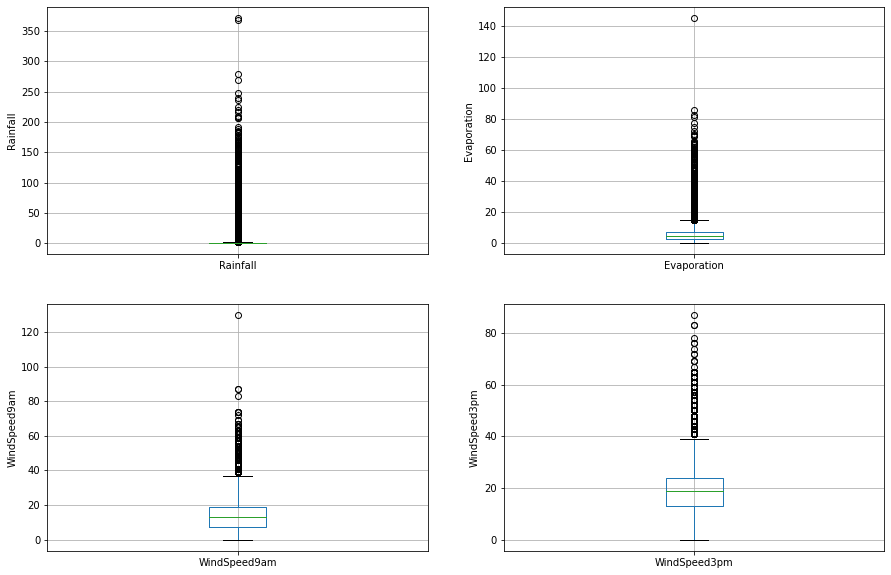
The above boxplots confirm that there are lot of outliers in these variables.

Check the distribution of variables

Now, I will plot the histograms to check distributions to find out if they are normal or skewed.

If the variable follows normal distribution, then I will do Extreme Value Analysis otherwise if they are skewed, I will find IQR (Interquantile range).

 1
 2
 3
 4
 5
 6
 7
 8
 9
10
11
12
13
14
15
16
17
18
19
20
21
22
23
24
25
26
27

# plot histogram to check distribution

plt.figure(figsize=(15,10))


plt.subplot(2, 2, 1)
fig = df.Rainfall.hist(bins=10)
fig.set_xlabel('Rainfall')
fig.set_ylabel('RainTomorrow')


plt.subplot(2, 2, 2)
fig = df.Evaporation.hist(bins=10)
fig.set_xlabel('Evaporation')
fig.set_ylabel('RainTomorrow')


plt.subplot(2, 2, 3)
fig = df.WindSpeed9am.hist(bins=10)
fig.set_xlabel('WindSpeed9am')
fig.set_ylabel('RainTomorrow')


plt.subplot(2, 2, 4)
fig = df.WindSpeed3pm.hist(bins=10)
fig.set_xlabel('WindSpeed3pm')
fig.set_ylabel('RainTomorrow')

Text(0, 0.5, 'RainTomorrow')

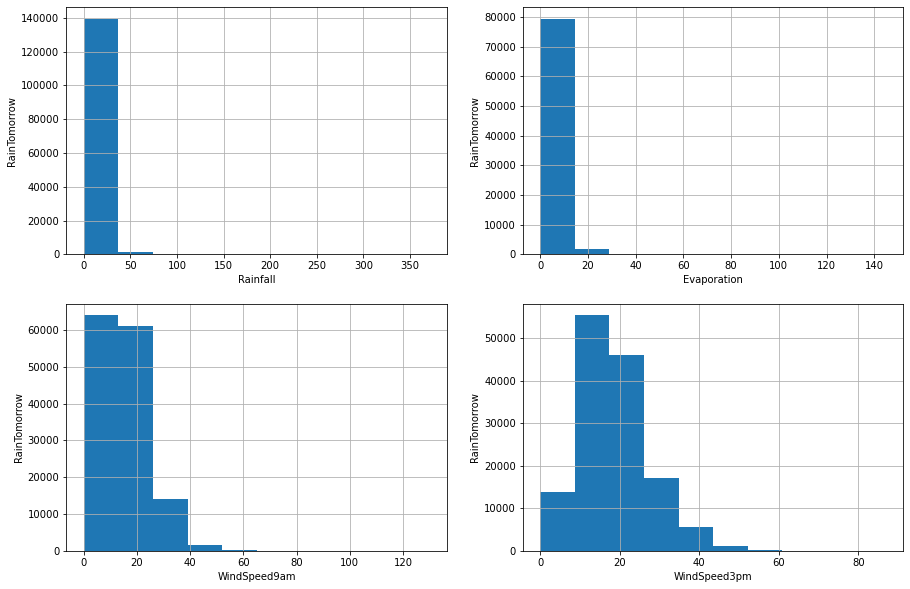
We can see that all the four variables are skewed. So, I will use interquantile range to find outliers

1
2
3
4
5
6

# find outliers for Rainfall variable

IQR = df.Rainfall.quantile(0.75) - df.Rainfall.quantile(0.25)
Lower_fence = df.Rainfall.quantile(0.25) - (IQR * 3)
Upper_fence = df.Rainfall.quantile(0.75) + (IQR * 3)
print(f'Rainfall outliers are values < {Lower_fence} or > {Upper_fence}')

Rainfall outliers are values < -2.4000000000000004 or > 3.2

For Rainfall, the minimum and maximum values are 0.0 and 371.0. So, the outliers are values > 3.2.

1
2
3
4
5
6

# find outliers for Evaporation variable

IQR = df.Evaporation.quantile(0.75) - df.Evaporation.quantile(0.25)
Lower_fence = df.Evaporation.quantile(0.25) - (IQR * 3)
Upper_fence = df.Evaporation.quantile(0.75) + (IQR * 3)
print(f'Evaporation outliers are values < {Lower_fence} or > {Upper_fence}')

Evaporation outliers are values < -11.800000000000002 or > 21.800000000000004

For Evaporation, the minimum and maximum values are 0.0 and 145.0. So, the outliers are values > 21.8.

1
2
3
4
5
6

# find outliers for WindSpeed9am variable

IQR = df.WindSpeed9am.quantile(0.75) - df.WindSpeed9am.quantile(0.25)
Lower_fence = df.WindSpeed9am.quantile(0.25) - (IQR * 3)
Upper_fence = df.WindSpeed9am.quantile(0.75) + (IQR * 3)
print(f'WindSpeed9am outliers are values < {Lower_fence} or > {Upper_fence}')

WindSpeed9am outliers are values < -29.0 or > 55.0

For WindSpeed9am, the minimum and maximum values are 0.0 and 130.0. So, the outliers are values > 55.0.

1
2
3
4
5
6

# find outliers for WindSpeed3pm variable

IQR = df.WindSpeed3pm.quantile(0.75) - df.WindSpeed3pm.quantile(0.25)
Lower_fence = df.WindSpeed3pm.quantile(0.25) - (IQR * 3)
Upper_fence = df.WindSpeed3pm.quantile(0.75) + (IQR * 3)
print(f'WindSpeed3pm outliers are values < {Lower_fence} or > {Upper_fence}')

WindSpeed3pm outliers are values < -20.0 or > 57.0

For WindSpeed3pm, the minimum and maximum values are 0.0 and 87.0. So, the outliers are values > 57.0.

Multivariate Analysis

• An important step in EDA is to discover patterns and relationships between variables in the dataset.
• I will use heat map and pair plot to discover the patterns and relationships in the dataset.
• First of all, I will draw a heat map.

1
2
3
4
5
6
7
8

correlation = df.corr()

plt.figure(figsize=(16,12))
plt.title('Correlation Heatmap of Rain in Australia Dataset')
ax = sns.heatmap(correlation, square=True, annot=True, fmt='.2f', linecolor='white')
ax.set_xticklabels(ax.get_xticklabels(), rotation=90)
ax.set_yticklabels(ax.get_yticklabels(), rotation=30)           
plt.show()

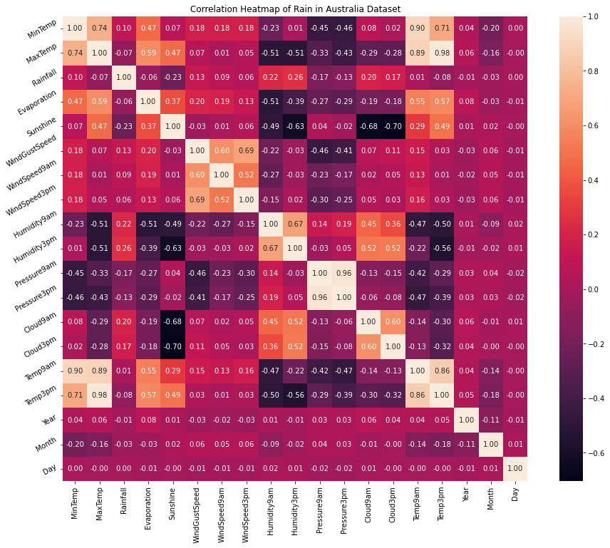
Interpretation

From the above correlation heat map, we can conclude that :

• MinTemp and MaxTemp variables are highly positively correlated (correlation coefficient = 0.74).
• MinTemp and Temp3pm variables are also highly positively correlated (correlation coefficient = 0.71).
• MinTemp and Temp9am variables are strongly positively correlated (correlation coefficient = 0.90).
• MaxTemp and Temp9am variables are strongly positively correlated (correlation coefficient = 0.89).
• MaxTemp and Temp3pm variables are also strongly positively correlated (correlation coefficient = 0.98).
• WindGustSpeed and WindSpeed3pm variables are highly positively correlated (correlation coefficient = 0.69).
• Pressure9am and Pressure3pm variables are strongly positively correlated (correlation coefficient = 0.96).
• Temp9am and Temp3pm variables are strongly positively correlated (correlation coefficient = 0.86).

Pair Plot

First of all, I will define extract the variables which are highly positively correlated.

1
2
3

num_var = ['MinTemp', 'MaxTemp', 'Temp9am', 'Temp3pm', 'WindGustSpeed', 'WindSpeed3pm', 'Pressure9am', 'Pressure3pm']
sns.pairplot(df[num_var], kind='scatter', diag_kind='hist', palette='Rainbow')
plt.show()

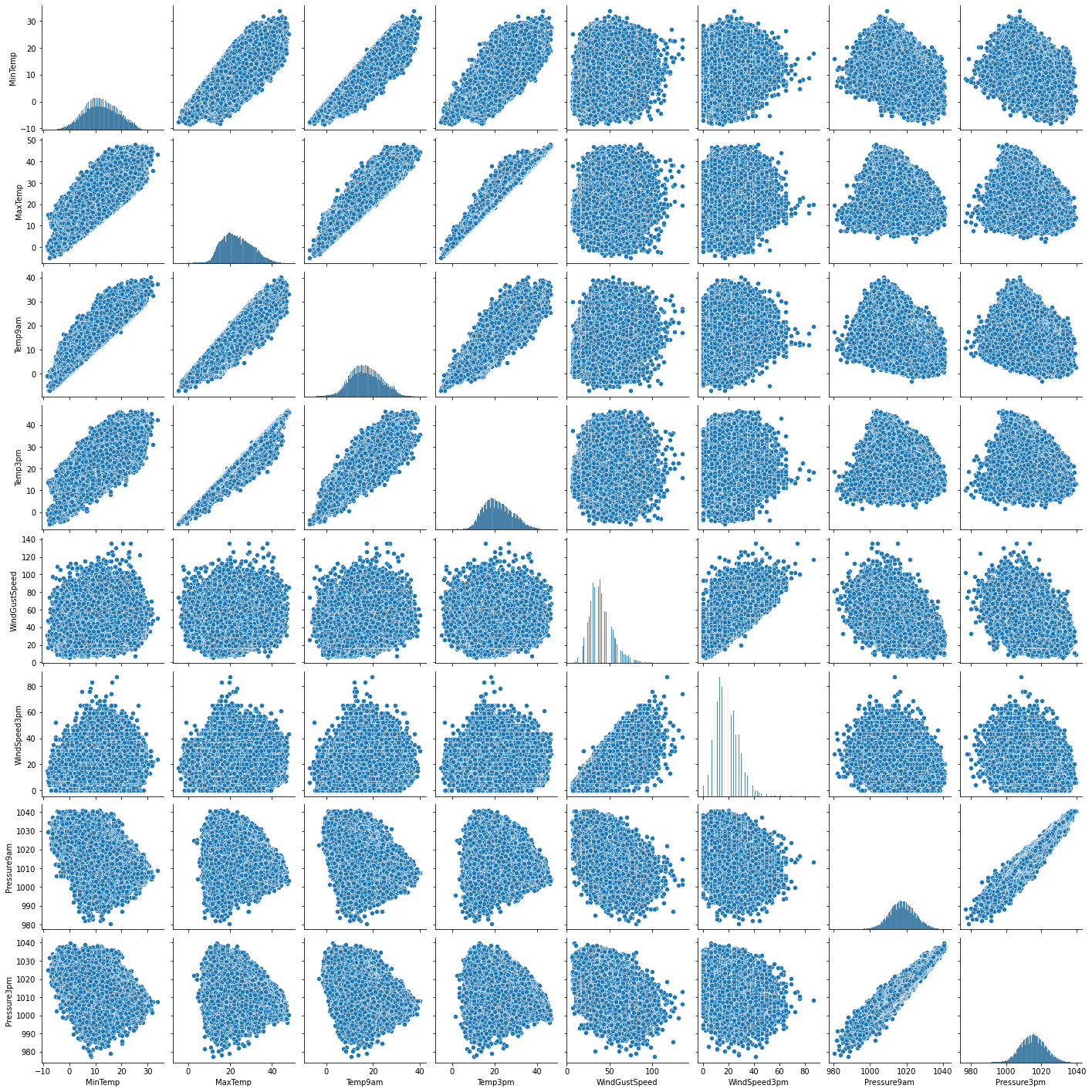
Interpretation

• I have defined a variable num_var which consists of MinTemp, MaxTemp, Temp9am, Temp3pm, WindGustSpeed, WindSpeed3pm, Pressure9am and Pressure3pm variables.
• The above pair plot shows relationship between these variables.

Split target from features

1
2
3
4
5

X = df.drop(['RainTomorrow'], axis=1)
y = df['RainTomorrow']

# split X and y into training and testing sets
X_train, X_test, y_train, y_test = train_test_split(X, y, test_size = 0.2, random_state = 42)

Feature Engineering

Feature Engineering is the process of transforming raw data into useful features that help us to understand our model better and increase its predictive power. I will carry out feature engineering on different types of variables.

Assumption

I assume that the data are missing completely at random (MCAR). There are two methods which can be used to impute missing values. One is mean or median imputation and other one is random sample imputation. When there are outliers in the dataset, we should use median imputation. So, I will use median imputation because median imputation is robust to outliers.

I will impute missing values with the appropriate statistical measures of the data, in this case median. Imputation should be done over the training set, and then propagated to the test set. It means that the statistical measures to be used to fill missing values both in train and test set, should be extracted from the train set only. This is to avoid overfitting.

1
2
3
4
5
6

# impute missing values in X_train and X_test with respective column median in X_train

for df1 in [X_train, X_test]:
    for col in numerical:
        col_median=X_train[col].median()
        df1[col].fillna(col_median, inplace=True)     

1
2
3

# check again missing values in numerical variables in X_train

X_train[numerical].isnull().sum()

MinTemp          0
MaxTemp          0
Rainfall         0
Evaporation      0
Sunshine         0
WindGustSpeed    0
WindSpeed9am     0
WindSpeed3pm     0
Humidity9am      0
Humidity3pm      0
Pressure9am      0
Pressure3pm      0
Cloud9am         0
Cloud3pm         0
Temp9am          0
Temp3pm          0
Year             0
Month            0
Day              0
dtype: int64

Engineering missing values in categorical variables

1
2
3
4
5
6
7

# impute missing categorical variables with most frequent value

for df2 in [X_train, X_test]:
    df2['WindGustDir'].fillna(X_train['WindGustDir'].mode()[0], inplace=True)
    df2['WindDir9am'].fillna(X_train['WindDir9am'].mode()[0], inplace=True)
    df2['WindDir3pm'].fillna(X_train['WindDir3pm'].mode()[0], inplace=True)
    df2['RainToday'].fillna(X_train['RainToday'].mode()[0], inplace=True)

1
2
3

# check missing values in categorical variables in X_train
categorical = X_train.select_dtypes(include=['object']).columns
X_train[categorical].isnull().sum()

Location       0
WindGustDir    0
WindDir9am     0
WindDir3pm     0
RainToday      0
dtype: int64

Engineering outliers in numerical variables

We have seen that the Rainfall, Evaporation, WindSpeed9am and WindSpeed3pm columns contain outliers. I will use top-coding approach to cap maximum values and remove outliers from the above variables.

1
2
3
4
5
6
7
8

def max_value(df3, variable, top):
    return np.where(df3[variable]>top, top, df3[variable])

for df3 in [X_train, X_test]:
    df3['Rainfall'] = max_value(df3, 'Rainfall', 3.2)
    df3['Evaporation'] = max_value(df3, 'Evaporation', 21.8)
    df3['WindSpeed9am'] = max_value(df3, 'WindSpeed9am', 55)
    df3['WindSpeed3pm'] = max_value(df3, 'WindSpeed3pm', 57)

Encode categorical variables

1
2
3

encoder = ce.BinaryEncoder(cols=['RainToday'])
X_train = encoder.fit_transform(X_train)
X_test = encoder.transform(X_test)

1
2

X_train = pd.get_dummies(X_train)
X_test = pd.get_dummies(X_test)

We now have training and testing set ready for model building. Before that, we should map all the feature variables onto the same scale. It is called feature scaling. I will do it as follows

1
2
3
4
5
6

cols = X_train.columns
scaler = MinMaxScaler()
X_train = scaler.fit_transform(X_train)
X_test = scaler.transform(X_test)
X_train = pd.DataFrame(X_train, columns=[cols])
X_test = pd.DataFrame(X_test, columns=[cols])

Now we can finally train the logistic regression model

Modelling

1
2
3
4

# instantiate the model
logreg = LogisticRegression(solver='liblinear', random_state=42)
# fit the model
logreg.fit(X_train, y_train)

LogisticRegression(random_state=42, solver='liblinear')

LogisticRegression(random_state=42, solver='liblinear')

1

y_pred_test = logreg.predict(X_test)

predict_proba method

predict_proba method gives the probabilities for the target variable(0 and 1) in this case, in array form.

1
2

# probability of getting output as 0 - no rain
logreg.predict_proba(X_test)[:,0]

array([0.15163563, 0.703692  , 0.98254885, ..., 0.98586207, 0.9495434 ,
       0.95416021])

1
2

# probability of getting output as 1 - rain
logreg.predict_proba(X_test)[:,1]

array([0.84836437, 0.296308  , 0.01745115, ..., 0.01413793, 0.0504566 ,
       0.04583979])

1

print(f'Model accuracy score: {accuracy_score(y_test, y_pred_test):0.4f}')

Model accuracy score: 0.8455

Compare the train-set and test-set accuracy

Now, I will compare the train-set and test-set accuracy to check for overfitting.

1
2

y_pred_train = logreg.predict(X_train)
print(f'Training-set accuracy score: {accuracy_score(y_train, y_pred_train):0.4f}')

Training-set accuracy score: 0.8483

The training-set accuracy score is 0.8483 while the test-set accuracy to be 0.8455. These two values are quite comparable. So, there is no question of overfitting.

In Logistic Regression, we use default value of C = 1 (C is the inverse of regularization strength, regularization wasn’t discussed in this article, maybe in another article in the future). It provides good performance with approximately 85% accuracy on both the training and the test set. But the model performance on both the training and test set are very comparable. It is likely the case of underfitting.

I will increase C and fit a more flexible model.

1
2
3
4

# fit the Logsitic Regression model with C=100
logreg100 = LogisticRegression(C=100, solver='liblinear', random_state=42)
# fit the model
logreg100.fit(X_train, y_train)

LogisticRegression(C=100, random_state=42, solver='liblinear')

LogisticRegression(C=100, random_state=42, solver='liblinear')

1
2
3

# print the scores on training and test set
print(f'Training set score: {logreg100.score(X_train, y_train):.4f}')
print(f'Test set score: {logreg100.score(X_test, y_test):.4f}')

Training set score: 0.8488
Test set score: 0.8456

We can see that, C=100 results in higher test set accuracy and also a slightly increased training set accuracy. So, we can conclude that a more complex model should perform better.

Compare model accuracy with null accuracy

So, the model accuracy is 0.8501. But, we cannot say that our model is very good based on the above accuracy. We must compare it with the null accuracy. Null accuracy is the accuracy that could be achieved by always predicting the most frequent class.

So, we should first check the class distribution in the test set.

1
2
3

# check class distribution in test set

y_test.value_counts()

No     22098
Yes     6341
Name: RainTomorrow, dtype: int64

We can see that the occurences of most frequent class is 22098. So, we can calculate null accuracy by dividing 22098 by total number of occurences.

1
2
3
4
5

# check null accuracy score

null_accuracy = (22098/(22098+6341))

print('Null accuracy score: {0:0.4f}'. format(null_accuracy))

Null accuracy score: 0.7770

Interpretation

We can see that our model accuracy score is 0.8501 but null accuracy score is 0.7759. So, we can conclude that our Logistic Regression model is doing a very good job in predicting the class labels.

Now, based on the above analysis we can conclude that our classification model accuracy is very good. Our model is doing a very good job in terms of predicting the class labels.

But, it does not give the underlying distribution of values. Also, it does not tell anything about the type of errors our classifer is making.

We have another tool called Confusion matrix that comes to our rescue.

Confusion matrix

A confusion matrix is a tool for summarizing the performance of a classification algorithm. A confusion matrix will give us a clear picture of classification model performance and the types of errors produced by the model. It gives us a summary of correct and incorrect predictions broken down by each category. The summary is represented in a tabular form.

Four types of outcomes are possible while evaluating a classification model performance. These four outcomes are described below:

• True Positives (TP) – True Positives occur when we predict an observation belongs to a certain class and the observation actually belongs to that class.

• True Negatives (TN) – True Negatives occur when we predict an observation does not belong to a certain class and the observation actually does not belong to that class.

• False Positives (FP) – False Positives occur when we predict an observation belongs to a certain class but the observation actually does not belong to that class. This type of error is called Type I error.

• False Negatives (FN) – False Negatives occur when we predict an observation does not belong to a certain class but the observation actually belongs to that class. This is a very serious error and it is called Type II error.

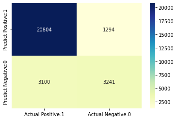
These four outcomes are summarized in a confusion matrix given below.

1
2
3
4
5
6

cm = confusion_matrix(y_test, y_pred_test)
print('Confusion matrix\n\n', cm)
print('\nTrue Positives(TP) = ', cm[0,0])
print('\nTrue Negatives(TN) = ', cm[1,1])
print('\nFalse Positives(FP) = ', cm[0,1])
print('\nFalse Negatives(FN) = ', cm[1,0])

Confusion matrix

 [[20804  1294]
 [ 3100  3241]]

True Positives(TP) =  20804

True Negatives(TN) =  3241

False Positives(FP) =  1294

False Negatives(FN) =  3100

The confusion matrix shows 20892 + 3285 = 24177 correct predictions and 3087 + 1175 = 4262 incorrect predictions.

In this case, we have

• True Positives (Actual Positive:1 and Predict Positive:1) - 20892
• True Negatives (Actual Negative:0 and Predict Negative:0) - 3285
• False Positives (Actual Negative:0 but Predict Positive:1) - 1175 (Type I error)
• False Negatives (Actual Positive:1 but Predict Negative:0) - 3087 (Type II error)

1
2
3
4

cm_matrix = pd.DataFrame(data=cm, columns=['Actual Positive:1', 'Actual Negative:0'], 
                                 index=['Predict Positive:1', 'Predict Negative:0'])

sns.heatmap(cm_matrix, annot=True, fmt='d', cmap='YlGnBu')

<AxesSubplot:>

Classification Metrices

Classification Report

Classification report is another way to evaluate the classification model performance. It displays the precision, recall, f1 and support scores for the model.

We can print a classification report as follows:

1

print(classification_report(y_test, y_pred_test))

              precision    recall  f1-score   support

          No       0.87      0.94      0.90     22098
         Yes       0.71      0.51      0.60      6341

    accuracy                           0.85     28439
   macro avg       0.79      0.73      0.75     28439
weighted avg       0.84      0.85      0.84     28439

1
2
3
4

TP = cm[0,0]
TN = cm[1,1]
FP = cm[0,1]
FN = cm[1,0]

Precision

Precision can be defined as the percentage of correctly predicted positive outcomes out of all the predicted positive outcomes. It can be given as the ratio of true positives (TP) to the sum of true and false positives (TP + FP).

So, Precision identifies the proportion of correctly predicted positive outcome. It is more concerned with the positive class than the negative class.

Mathematically, precision can be defined as the ratio of TP to (TP + FP).

1
2
3
4

# print precision score

precision = TP / float(TP + FP)
print('Precision : {0:0.4f}'.format(precision))

Precision : 0.9414

Recall

Recall can be defined as the percentage of correctly predicted positive outcomes out of all the actual positive outcomes. It can be given as the ratio of true positives (TP) to the sum of true positives and false negatives (TP + FN). Recall is also called Sensitivity.

Recall identifies the proportion of correctly predicted actual positives.

Mathematically, recall can be given as the ratio of TP to (TP + FN).

1
2

recall = TP / float(TP + FN)
print('Recall or Sensitivity : {0:0.4f}'.format(recall))

Recall or Sensitivity : 0.8703

1
2

specificity = TN / (TN + FP)
print('Specificity : {0:0.4f}'.format(specificity))

Specificity : 0.7147

f1-score

f1-score is the weighted harmonic mean of precision and recall. The best possible f1-score would be 1.0 and the worst would be 0.0. f1-score is the harmonic mean of precision and recall. So, f1-score is always lower than accuracy measures as they embed precision and recall into their computation. The weighted average of f1-score should be used to compare classifier models, not global accuracy.

Support

Support is the actual number of occurrences of the class in our dataset

1
2
3
4
5

# print the first 10 predicted probabilities of two classes- 0 and 1

y_pred_prob = logreg.predict_proba(X_test)[0:10]

y_pred_prob

array([[0.15163563, 0.84836437],
       [0.703692  , 0.296308  ],
       [0.98254885, 0.01745115],
       [0.86912045, 0.13087955],
       [0.61398609, 0.38601391],
       [0.94498646, 0.05501354],
       [0.95470402, 0.04529598],
       [0.5290216 , 0.4709784 ],
       [0.99863574, 0.00136426],
       [0.78819565, 0.21180435]])

Observations

• In each row, the numbers sum to 1.

• There are 2 columns which correspond to 2 classes - 0 and 1.

  • Class 0 - predicted probability that there is no rain tomorrow.
  • Class 1 - predicted probability that there is rain tomorrow.

• Importance of predicted probabilities

  • We can rank the observations by probability of rain or no rain.

• predict_proba process

  • Predicts the probabilities
  • Choose the class with the highest probability

• Classification threshold level

  • There is a classification threshold level of 0.5.
  • Class 1 - probability of rain is predicted if probability > 0.5.
  • Class 0 - probability of no rain is predicted if probability < 0.5.

1
2
3
4
5

# store the probabilities in dataframe
y_pred_prob_df = pd.DataFrame(data=y_pred_prob, columns=['Prob of - No rain tomorrow (0)', 'Prob of - Rain tomorrow (1)'])

# store the predicted probabilities for class 1 - Probability of rain
y_pred1 = logreg.predict_proba(X_test)[:, 1]

 1
 2
 3
 4
 5
 6
 7
 8
 9
10
11
12
13
14
15
16

# plot histogram of predicted probabilities
# adjust the font size 
plt.rcParams['font.size'] = 12

# plot histogram with 10 bins
plt.hist(y_pred1, bins = 10)

# set the title of predicted probabilities
plt.title('Histogram of predicted probabilities of rain')

# set the x-axis limit
plt.xlim(0,1)

# set the title
plt.xlabel('Predicted probabilities of rain')
plt.ylabel('Frequency')

Text(0, 0.5, 'Frequency')

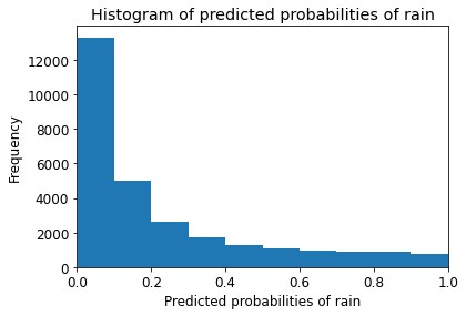
Observations

• We can see that the above histogram is highly positive skewed.
• The first column tell us that there are approximately 15000 observations with probability between 0.0 and 0.1.
• There are small number of observations with probability > 0.5.
• So, these small number of observations predict that there will be rain tomorrow.
• Majority of observations predict that there will be no rain tomorrow.

And that’s about it. Thank you for reading and see you in the next article!