This article goes in detail through one of the data science projects I worked on, the New York Taxi dataset which is made available by the New York City Taxi and Limousine Commission (TLC). New York is partly known for its yellow taxis (even though there are green taxis we’ll focus on only the yellow taxis) and there are millions of taxi rides taken every month as New York is one of the most populous cities in the United States which makes for a very interesting dataset to dive into as there are a lot of analysis possibilities (Geospatial Data Analysis, Time Analysis, Taxi Ride Price Analysis, Traffic Analysis, etc.).
Introduction
When seen as a whole, the precise trip-level data is more than simply a long list of taxi pickup and drop-off locations: it tells a tale of New York. How much do taxis make each trip if they can only travel 30 or 50 kilometres per trip, as opposed to taxis with no limit? Is it more common for taxi journeys to begin in the north or south? What is the average speed of New York traffic (with regards to taxis)? How does the speed of traffic in New York change during the day? All of these questions, and many more, are addressed in the dataset. And we will answer them as well as others.
The Process
The usual data science process starts with business and feasability study, data collection, data cleaning, exploratory data analysis (EDA) and sometimes modelling. Of course there is more to this simple process abstraction, such as model deployment and monitoring but in our case these are skipped as we will focus on the data collection, cleaning and exploratory analysis. We’ll now go through the different phases one by one.
Data Collection
The data is taken from this link: NYC Yellow Taxi provided by Andrés Monroy. The link contains data contains compressed files of yellow taxi rides for the year 2013. There are two compressed files one named trip_data is for trip specific data such as the distance, time, etc while the other one named trip_fare contains data regarding the trip fare (hence the name), surcharge, tip, etc. Both files divide the data in 12 CSV files (one for each month). The data is also available in Kaggle for the trip data and trip fare here and here respectively. Kaggle wasn’t used as it doesn’t contain all the data (even though we are also not using all of it, more below) and for the fare data the data is shuffled between several years. The data dictionary/description can be found here: Data Dictionary, note that not all columns are in the data dictionary from the data source somehow but looking further in the analysis they are all made clear and are mostly Intuitive.
After downloading the compressed files and unzipping them they are about 5.4 GB in total, which is quite hefty for my local machine as I am doing the analysis locally on a small machine and not on the cloud. This is where data sampling comes into play. Reservoir random sampling was used to sample 150K records/trips per month of 2013. The code for this is shown here and is also available in the projects github repo.
importpandasaspdimportnumpyasnpimportosfromitertoolsimportislicefromioimportStringIOfromtqdm.notebookimporttqdmpd.set_option("display.max_columns",None)np.random.seed(42)defreservoir_sample(iterable,random1,random2,random3,random4,k=1):'''
From : https://en.wikipedia.org/wiki/Reservoir_sampling#An_optimal_algorithm
'''iterator=iter(iterable)values=list(islice(iterator,k))W=np.exp(np.log(random1/k))whileTrue:skip=int(np.floor(np.log(random2)/np.log(1-W)))selection=list(islice(iterator,skip,skip+1))ifselection:values[random3]=selection[0]W*=np.exp(np.log(random4)/k)else:returnvaluesdefdf_sample(filepath1,filepath2,k):r1,r2,r3,r4=np.random.random(),np.random.random(),np.random.randint(k),np.random.random()withopen(filepath1,'r')asf1,open(filepath2,'r')asf2:header1=next(f1)header2=next(f2)values1=reservoir_sample(f1,r1,r2,r3,r4,k)values2=reservoir_sample(f2,r1,r2,r3,r4,k)result1=[header1]+values1result2=[header2]+values2df1=pd.read_csv(StringIO(''.join(result1)))df2=pd.read_csv(StringIO(''.join(result2)))df1=sample_preprocessing(df1)df2=sample_preprocessing(df2,fare=True)#f2 has to be fare datareturndf1,df2defsample_preprocessing(df_sample,fare=False):df_sample.columns=df_sample.columns.str.replace(" ","")iffare:df_sample.drop(columns=["hack_license","vendor_id"],inplace=True)returndf_sampledefreduce_memory(df,verbose=True):numerics=["int8","int16","int32","int64","float16","float32","float64"]start_mem=df.memory_usage().sum()/1024**2forcolindf.columns:col_type=df[col].dtypesifcol_typeinnumerics:c_min=df[col].min()c_max=df[col].max()ifstr(col_type)[:3]=="int":ifc_min>np.iinfo(np.int8).minandc_max<np.iinfo(np.int8).max:df[col]=df[col].astype(np.int8)elifc_min>np.iinfo(np.int16).minandc_max<np.iinfo(np.int16).max:df[col]=df[col].astype(np.int16)elifc_min>np.iinfo(np.int32).minandc_max<np.iinfo(np.int32).max:df[col]=df[col].astype(np.int32)elifc_min>np.iinfo(np.int64).minandc_max<np.iinfo(np.int64).max:df[col]=df[col].astype(np.int64)else:if(c_min>np.finfo(np.float16).minandc_max<np.finfo(np.float16).max):df[col]=df[col].astype(np.float16)elif(c_min>np.finfo(np.float32).minandc_max<np.finfo(np.float32).max):df[col]=df[col].astype(np.float32)else:df[col]=df[col].astype(np.float64)end_mem=df.memory_usage().sum()/1024**2ifverbose:print("Mem. usage decreased to {:.2f} Mb ({:.1f}% reduction)".format(end_mem,100*(start_mem-end_mem)/start_mem))returndfdata_file_list=sorted(os.listdir("../Data/NYC Trip Data/"),key=lambdax:int(x.split(".")[0].split("_")[-1]))data_file_list=[os.path.join("../Data/NYC Trip Data/",file)forfileindata_file_list]fare_file_list=sorted(os.listdir("../Data/NYC Trip Fare/"),key=lambdax:int(x.split(".")[0].split("_")[-1]))fare_file_list=[os.path.join("../Data/NYC Trip Fare/",file)forfileinfare_file_list]N=150000# Number of records per month chosen randomly df_data=[]df_fare=[]zipped_data=zip(data_file_list,fare_file_list)fordata_file,fare_fileintqdm(zipped_data,total=len(data_file_list)):df_data_sample,df_fare_sample=df_sample(data_file,fare_file,N)df_data.append(df_data_sample)df_fare.append(df_fare_sample)fare=pd.concat(df_fare,axis=0,ignore_index=True)data=pd.concat(df_data,axis=0,ignore_index=True)data.drop_duplicates(subset=["medallion","pickup_datetime"],inplace=True)fare.drop_duplicates(subset=["medallion","pickup_datetime"],inplace=True)final_df=data.merge(fare,how="inner",on=["medallion","pickup_datetime"])final_df["pickup_datetime"]=pd.to_datetime(final_df["pickup_datetime"])final_df["dropoff_datetime"]=pd.to_datetime(final_df["dropoff_datetime"])final_df.to_csv("../Data/Pre-processed Data/data.csv")
The main sampling is conducted in the df_sample function which utilizes the reservoir sampling function itself. The main idea of reservoir sampling is explained here along with the pseudocode for its implementation. What we need to know is that it chooses a random sample (row) without replacement from the CSV file in a single pass over the whole file. Finally the fare and trip data are then joined together on the trips medallion and pickup datatime as they the represent the same trip just different data which gives us the final data to work with. It has about 2 million records (1.8M to be exact).
Data Cleaning
In this phase of the project we’ll check the data for any inconsistencies, outliers, erroneous values, etc. The cleaning itself is divided into several parts such as location data (pickup, dropoff) cleaning, trip duration cleaning, trip distance cleaning, trip speed cleaning, trip total amount, fare Amount, surcharge, tax, tolls and tip cleaning and categorical columns cleaning. We’ll also use this phase to calculate and add some other features/columns as well. Let’s get straight to it 😍!
count 1770605
mean 0 days 00:12:17.623533763
std 0 days 00:11:57.343927277
min 0 days 00:00:00
25% 0 days 00:06:00
50% 0 days 00:10:00
75% 0 days 00:16:00
max 7 days 01:13:13
dtype: object
We’re seeing weird trip durations of 7 days and 0 seconds here.
Here we correct the invalid trip duration by calculating it from the pickup and dropoff datetime as well as remove the negative and trips with zero seconds. We do that using numpy’s np.where to get all the rows where the duration is invalid and correct that in line 6. We finally add the trip duration in minutes as well.
count 1768663
mean 0 days 00:12:18.433447751
std 0 days 00:11:57.320887829
min 0 days 00:00:01
25% 0 days 00:06:00
50% 0 days 00:10:00
75% 0 days 00:16:00
max 7 days 01:13:13
dtype: object
We corrected the incorrect trip duration, removed the zero and negative duration trips but we still see very low trip durations of 1 second and very high trip duration of 7 days. We can inspect the percentiles of the trip duration distribution to get an idea where to cut the maximum and minimum values.
before=df.shape[0]print(f'Rows/Size Before: {before}')invalid_distance_idx=df[(df.trip_distance>100)|(df.trip_distance==0)].index.tolist()# Remove distance of 0 and greater than 100 miles https://www.google.com/maps/dir/40.5055432,-74.2381798/41.0191685,-73.7871866/@40.9358817,-74.3487811,8.92z/data=!3m1!5s0x89c2f2be234865c9:0x12533050f3f45b3c!4m2!4m1!3e0df.drop(invalid_distance_idx,inplace=True)df.reset_index(drop=True,inplace=True)after=df.shape[0]print(f'Rows/Size After: {after}')print(f'Removed: {before-after}')
speeds=df["trip_speed_mi/hr"].valuesspeeds=np.sort(speeds,axis=None)foriinnp.arange(0.0,1.0,0.1):print("{} percentile is {}".format(99+i,speeds[int(len(speeds)*(float(99+i)/100))]))print("100 percentile value is ",speeds[-1])delspeeds
99.0 percentile is 37.835
99.1 percentile is 38.4
99.2 percentile is 39.025
99.3 percentile is 39.729
99.4 percentile is 40.518
99.5 percentile is 41.4
99.6 percentile is 42.45
99.7 percentile is 43.722
99.8 percentile is 45.408
99.9 percentile is 48.027
100 percentile value is 7280.0
1
2
3
4
5
6
7
8
before=df.shape[0]print(f'Rows/Size Before: {before}')df=df[(df["trip_speed_mi/hr"]>0)&(df["trip_speed_mi/hr"]<=50)].reset_index(drop=True)# 99.9th percentile is 48.027after=df.shape[0]print(f'Rows/Size After: {after}')print(f'Removed: {before-after}')
totals=df["total_amount"].valuestotals=np.sort(totals,axis=None)foriinnp.arange(0.0,1.0,0.1):print("{} percentile is {}".format(99+i,totals[int(len(totals)*(float(99+i)/100))]))print("100 percentile value is ",totals[-1])deltotals
99.0 percentile is 65.6
99.1 percentile is 67.7
99.2 percentile is 67.93
99.3 percentile is 68.23
99.4 percentile is 68.23
99.5 percentile is 69.38
99.6 percentile is 70.33
99.7 percentile is 72.28
99.8 percentile is 78.0
99.9 percentile is 91.66
100 percentile value is 563.12
df["passenger_count"].describe().apply(lambdax:'%.5f'%x)# Looks clean but we have passenger counts of 0
count 1764321.00000
mean 2.02239
std 1.65448
min 0.00000
25% 1.00000
50% 1.00000
75% 2.00000
max 6.00000
Name: passenger_count, dtype: object
1
2
3
print(df[df['passenger_count']==0].shape[0])#7 trips with passenger count 0, replace with mean valuedf.loc[df[df['passenger_count']==0].index,'passenger_count']=df.passenger_count.mean()
df.rate_code.unique()# Should only be 1,2,3,4,5,6 from data description, See: https://www1.nyc.gov/assets/tlc/downloads/pdf/data_dictionary_trip_records_yellow.pdf
We can use the Folium library to plot maps with markers and lines on it (and much more). We’ll use it to inspect some of these (14) abnormal rate code (rate code = 0) trips
They all look as expected so we finally save our clean dataset and onto EDA!
Data Analysis
Exploratory Data Analysis is the process of studying data and extracting insights from it in order to examine its major properties. EDA may be accomplished through the use of statistics and graphical approaches (using my favourite plotting library Plotly! With a bit of matplotlib as well 😁). Why is it important? We simply can’t make sense of such huge datasets if we don’t explore the data. Exploratory Data Analysis helps us look deeper and see if our intuition matches with the data. It helps us see if we are asking the right questions. Exploring and analyzing the data is important to see how features are distributed or if and how they are related with each other. How they are contributing to the target variable (varable to be predicted/modelled), if there is any or simply analyzing the features without it. This will eventually help us answer the questions we have around the dataset, allow us to formulate new questions and check if we are even asking the right questions. So let’s start as usual by importing and loading our the cleaned dataset.
df['pickup_datetime']=pd.to_datetime(df['pickup_datetime'])df['dropoff_datetime']=pd.to_datetime(df['dropoff_datetime'])# Too many addresses to geocode, Nominatim usage policy doesn't allow bulk geocoding and will timeout (was going to be used in hover)#df["pickup_address"] = df.apply(lambda x: geolocator.reverse(str(x.pickup_latitude) + "," + str(x.pickup_longitude),timeout=5)[0],axis=1)#df["dropoff_address"] = df.apply(lambda x: geolocator.reverse(str(x.dropoff_latitude) + "," + str(x.dropoff_longitude),timeout=5)[0],axis=1)
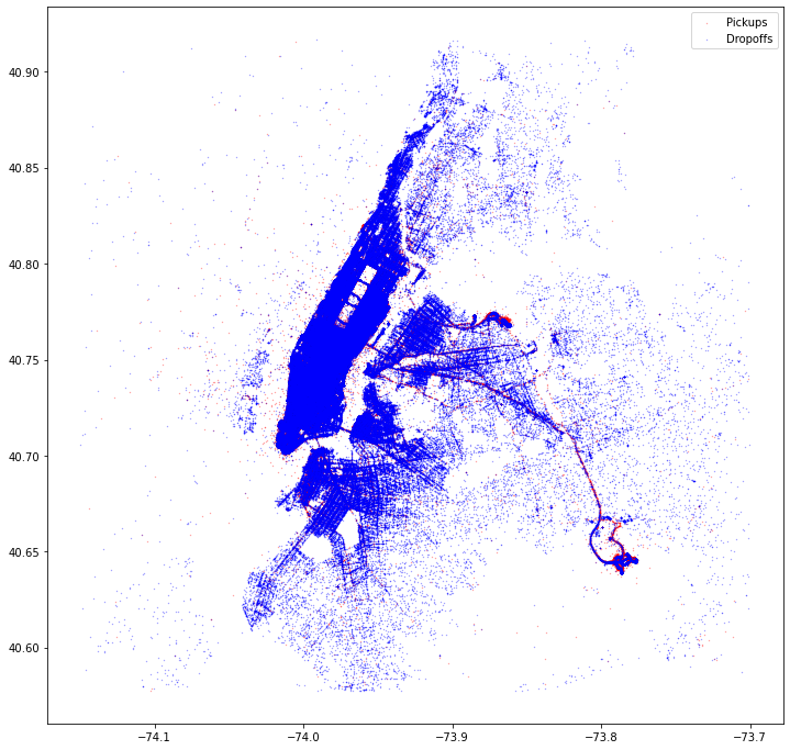
drop_pick_map(df_train,NYBB,title='Map of Pickups & Dropoffs',sample_size=10000)
We see a slight difference where the pickups are more on the West of New York in the Manhattan area but the dropoffs are more to the East of New York in the Queens and Brooklyn area.
We can also see all the pickups and dropoffs in one graphic below
1
all_hires(df_train,NYBB)
We’ll segment the EDA sections by question and we’ll start with our first question
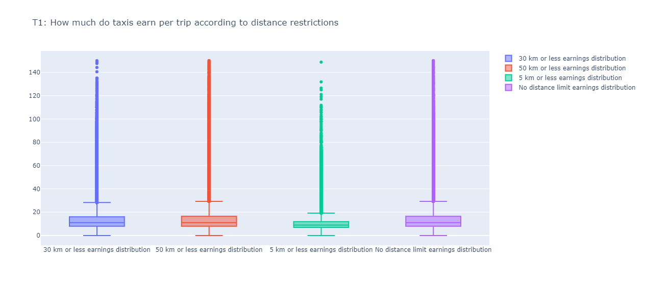
Q1: How much do taxis earn per trip if they can only drive 30km or 50km per trip, compared to taxis that have no limit? (i.e. what is the average income for trips <30km or <50km compared to the total revenue?)
1
2
3
4
5
6
7
8
9
10
11
12
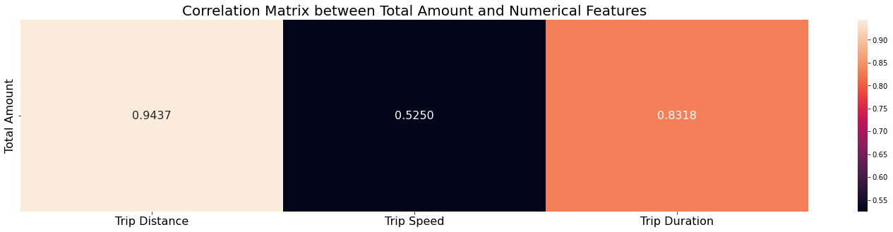
columns=['trip_distance','trip_speed_mi/hr','trip_time_in_secs']correlation_amount=pd.DataFrame(index=["total_amount"],columns=columns)fori,colinenumerate(columns):cor=df_train.total_amount.corr(df_train[col])correlation_amount.loc[:,columns[i]]=corplt.figure(figsize=(25,5))g=sns.heatmap(correlation_amount,annot=True,fmt='.4f',annot_kws={"fontsize":16})g.set_yticklabels(['Tip Amount'],fontsize=16)g.set_xticklabels(['Trip Distance','Trip Speed','Trip Duration'],fontsize=16)g.set_yticklabels(['Total Amount'],fontsize=16)plt.title("Correlation Matrix between Total Amount and Numerical Features",fontdict={'fontsize':20})plt.plot()
Total Amount is highly positively correlated with the trip distance (0.94) and trip duration (0.83)
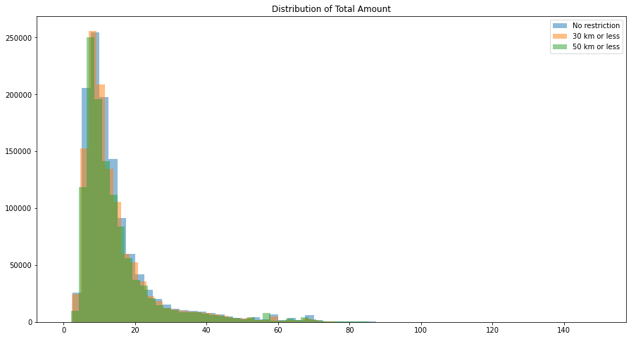
Significant Difference between Trips less than 5km and all trips, no significant difference from the other restrictions, this is mainly due to the fact that <30km and <50km capture most trips
We can also see the difference below in the box plots and histograms
print("Mean Total Amount for 30 km or less: ",df_30_less.total_amount.mean())print("Mean Total Amount for 50 km or less: ",df_50_less.total_amount.mean())print("Mean Total Amount for 5 km or less: ",df_5_less.total_amount.mean())print("Mean Total Amount for no distance restriction: ",df_train.total_amount.mean())
Mean Total Amount for 30 km or less: 14.223142284432392
Mean Total Amount for 50 km or less: 14.645665338921816
Mean Total Amount for 5 km or less: 9.734024318446
Mean Total Amount for no distance restriction: 14.6549403897318
1
2
3
4
5
6
7
8
9
10
fig=go.Figure()fig.add_trace(go.Box(y=df_30_less["total_amount"],name="30 km or less earnings distribution"))fig.add_trace(go.Box(y=df_50_less["total_amount"],name="50 km or less earnings distribution"))fig.add_trace(go.Box(y=df_5_less["total_amount"],name="5 km or less earnings distribution"))fig.add_trace(go.Box(y=df_train["total_amount"],name="No distance limit earnings distribution"))fig=fig.update_layout(title="T1: How much do taxis earn per trip according to distance restrictions")fig.write_html("../Figures/T1/T1_fig.html")
1
2
3
4
5
6
7
8
9
10
11
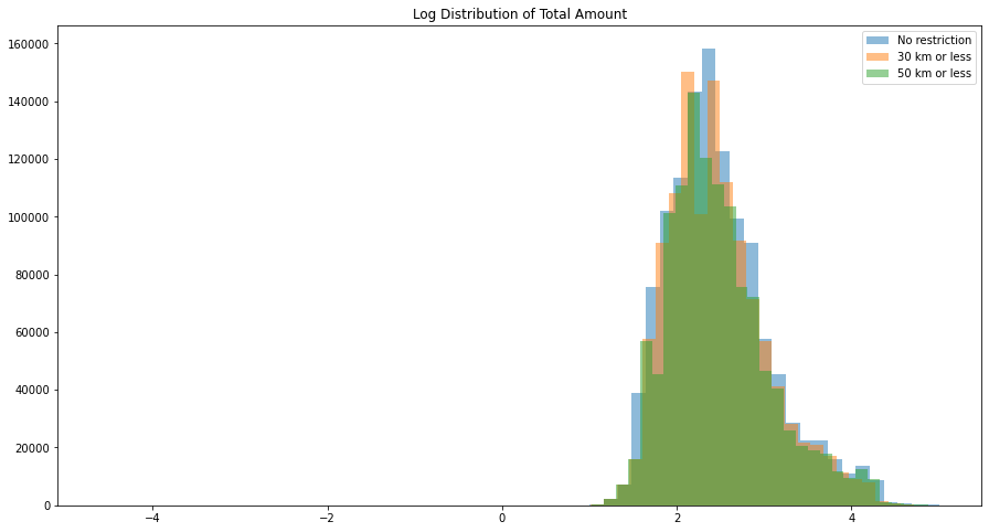
all_log=np.log(df_train.total_amount.values)km30_log=np.log(df_30_less.total_amount.values)km50_log=np.log(df_50_less.total_amount.values)fig=plt.figure(figsize=(15,8))plt.title("Log Distribution of Total Amount")plt.hist(all_log[np.isfinite(all_log)],bins=60,label='No restriction',alpha=0.5)plt.hist(km30_log[np.isfinite(km30_log)],bins=65,label='30 km or less',alpha=0.5)plt.hist(km50_log[np.isfinite(km50_log)],bins=70,label='50 km or less',alpha=0.5)plt.legend(loc='upper right')plt.show()
1
2
3
4
5
6
7
fig=plt.figure(figsize=(15,8))plt.title("Distribution of Total Amount")plt.hist(df_train.total_amount.values,bins=60,label='No restriction',alpha=0.5)plt.hist(df_30_less.total_amount.values,bins=65,label='30 km or less',alpha=0.5)plt.hist(df_50_less.total_amount.values,bins=70,label='50 km or less',alpha=0.5)plt.legend(loc='upper right')plt.show()
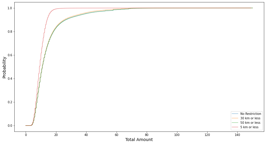
Kolmogorov–Smirnov Test is used to test for the significance in the difference between the distributions and again same results are observed analytically
1
2
3
4
5
6
7
8
ks_30vs_all=ss.ks_2samp(df_train['total_amount'].values,df_30_less['total_amount'].values)ks_50vs_all=ss.ks_2samp(df_train['total_amount'].values,df_50_less['total_amount'].values)ks_5vs_all=ss.ks_2samp(df_train['total_amount'].values,df_5_less['total_amount'].values)print(f"KS-Statistics between 30 km restriction and no restriction: {ks_30vs_all.statistic}, p-value: {ks_30vs_all.pvalue}")print(f"KS-Statistics between 50 km restriction and no restriction: {ks_50vs_all.statistic}, p-value: {ks_50vs_all.pvalue}")print(f"KS-Statistics between 5 km restriction and no restriction: {ks_5vs_all.statistic}, p-value: {ks_5vs_all.pvalue}")
KS-Statistics between 30 km restriction and no restriction:
0.008042675652436548, p-value: 1.6896187294453e-33
KS-Statistics between 50 km restriction and no restriction:
0.00011191457137738059, p-value: 1.0
KS-Statistics between 5 km restriction and no restriction:
0.23128162369336924, p-value: 0.0
The Kolmogorov–Smirnov Test is based on the cumulative distribution so we will look at that
 1
 2
 3
 4
 5
 6
 7
 8
 9
10
11
12
13
14
ecdf_norestrict=ECDF(df_train.total_amount.values)ecdf_30=ECDF(df_30_less.total_amount.values)ecdf_50=ECDF(df_50_less.total_amount.values)ecdf_5=ECDF(df_5_less.total_amount.values)fig=plt.figure(figsize=(15,8))plt.plot(ecdf_norestrict.x,ecdf_norestrict.y,label='No Restriction',alpha=0.5)plt.plot(ecdf_30.x,ecdf_30.y,label='30 km or less',alpha=0.5)plt.plot(ecdf_50.x,ecdf_50.y,label='50 km or less',alpha=0.5)plt.plot(ecdf_5.x,ecdf_5.y,label='5 km or less',alpha=0.5)_=plt.xlabel('Total Amount',fontdict=dict(size=14))_=plt.ylabel('Probability',fontdict=dict(size=14))plt.legend()plt.show()
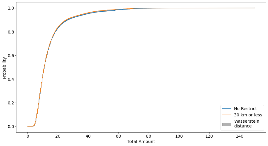
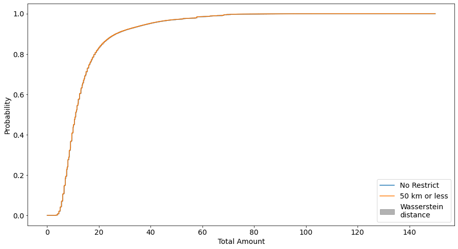
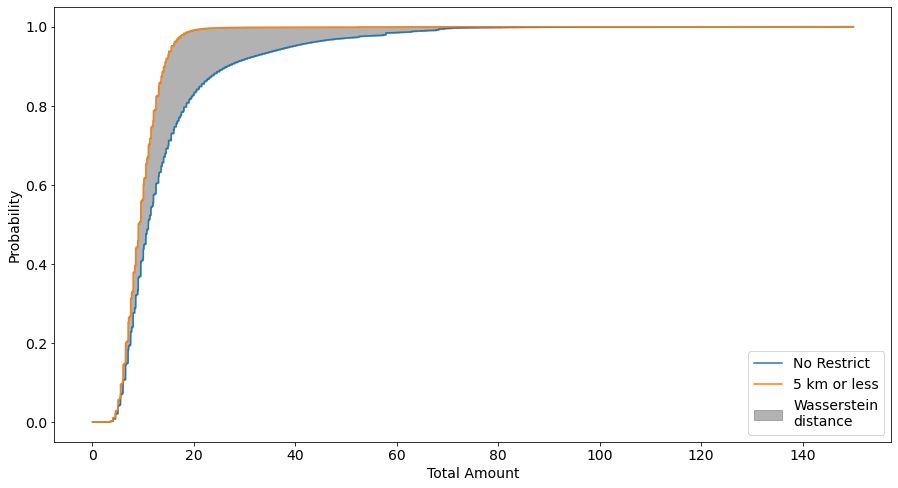
Another metric we can use to quanitfy the difference in the distributions is the Wasserstein Distance, which we inspect below visually and analytically
defwassersteindist_plot(a,b):all_values=sorted(set(a)|set(b))a_cdf=np.vstack([[np.mean(a<v)forvinall_values],[np.mean(a<=v)forvinall_values]]).flatten("F")b_cdf=np.vstack([[np.mean(b<v)forvinall_values],[np.mean(b<=v)forvinall_values]]).flatten("F")all_values=np.repeat(all_values,2)returnall_values,a_cdf,b_cdfav,cdf_all,cdf_30=wassersteindist_plot(df_train.total_amount.values,df_30_less.total_amount.values)av,cdf_all,cdf_50=wassersteindist_plot(df_train.total_amount.values,df_50_less.total_amount.values)av,cdf_all,cdf_5=wassersteindist_plot(df_train.total_amount.values,df_5_less.total_amount.values)fig,ax=plt.subplots(figsize=(15,8))ax.plot(av,cdf_all,label="No Restrict")ax.plot(av,cdf_30,label="30 km or less")ax.fill_between(av,cdf_all,cdf_30,color="grey",alpha=0.6,label="Wasserstein\ndistance")ax.tick_params(axis='both',which='major',labelsize=14)ax.set_xlabel('Total Amount',fontsize=14)ax.set_ylabel('Probability',fontsize=14)ax.legend(fontsize=14,loc="lower right")
1
2
3
4
5
6
7
8
9
fig,ax=plt.subplots(figsize=(15,8))ax.plot(av,cdf_all,label="No Restrict")ax.plot(av,cdf_50,label="50 km or less")ax.fill_between(av,cdf_all,cdf_50,color="grey",alpha=0.6,label="Wasserstein\ndistance")ax.tick_params(axis='both',which='major',labelsize=14)ax.set_xlabel('Total Amount',fontsize=14)ax.set_ylabel('Probability',fontsize=14)ax.legend(fontsize=14,loc="lower right")
1
2
3
4
5
6
7
8
9
fig,ax=plt.subplots(figsize=(15,8))ax.plot(av,cdf_all,label="No Restrict")ax.plot(av,cdf_5,label="5 km or less")ax.fill_between(av,cdf_all,cdf_5,color="grey",alpha=0.6,label="Wasserstein\ndistance")ax.tick_params(axis='both',which='major',labelsize=14)ax.set_xlabel('Total Amount',fontsize=14)ax.set_ylabel('Probability',fontsize=14)ax.legend(fontsize=14,loc="lower right")
Again from the wasserstein distance plots we see the same result, no significant difference (low wasserstein distance) between trips of less than 30 or 50km and all trips, but the opposite (high wasserstein distance) between trips of less than 5km and all trips.
We’ll also look at the standerdized wasserstein distance
defstandardized_wasserstein_distance(u,v,method="std"):u,v=np.array(u),np.array(v)numerator=ss.wasserstein_distance(u,v)concat=np.concatenate([u,v])ifmethod=='std':denominator=np.std(concat)elifmethod=='minmax':denominator=np.max(concat)-np.min(concat)elifmethod=='mean':denominator=max(np.max(concat)-np.mean(concat),np.mean(concat)-np.min(concat))elifmethod=='median':denominator=max(np.min(concat)-np.median(concat),np.median(concat)-np.min(concat))elifmethod=='iqr':denominator=np.diff(np.quantile(concat,[.25,.75]))[0]returnnumerator/denominatorifdenominator!=.0else.0print(f"SWD (mean method) between No Restriction and 30 km or less: {standardized_wasserstein_distance(df_train.total_amount.values,df_30_less.total_amount.values,method='mean')}")print(f"SWD (mean method) between No Restriction and 50 km or less: {standardized_wasserstein_distance(df_train.total_amount.values,df_50_less.total_amount.values,method='mean')}")print(f"SWD (mean method) between No Restriction and 5 km or less: {standardized_wasserstein_distance(df_train.total_amount.values,df_5_less.total_amount.values,method='mean')}")
SWD (mean method) between No Restriction and 30 km or less:
0.0031855750868686784
SWD (mean method) between No Restriction and 50 km or less:
6.868595381679189e-05
SWD (mean method) between No Restriction and 5 km or less:
0.035809828654724
Trip Distance matters!
Obviously as we have seen severe restrictions on distance affect the total trip amount and as seen in the correlation chart above, the trip distance is highly positevely correlated with the total amount
Q2: Do more taxi trips start at the North or South?
By taking a arbitrary north and south cutoff we get these results
1
2
3
4
5
south=df_train[df_train.pickup_latitude<40.66240321639479].reset_index(drop=True)north=df_train[df_train.pickup_latitude>40.803265534217225].reset_index(drop=True)print("Number of trips starting in the south: ",south.shape[0])print("Number of trips starting in the north: ",north.shape[0])
Number of trips starting in the south: 21708
Number of trips starting in the north: 19359
By taking the center of Manhatten as a cutoff we get a more intutive answer
1
2
3
4
5
south2=df_train[df_train.pickup_latitude<40.78035634806236].reset_index(drop=True)north2=df_train[df_train.pickup_latitude>40.78035634806236].reset_index(drop=True)print("Number of trips starting in the south: ",south2.shape[0])print("Number of trips starting in the north: ",north2.shape[0])
Number of trips starting in the south: 1062763
Number of trips starting in the north: 119332
Some trips are in water! These will be removed and numbers checked again (should have been done in the cleaning phase but these weren’t detected until now)
BB=(-74.5,-72.8,40.5,41.8)nyc_water=plt.imread('water_mask.png')[:,:,0]>0.9# Mask defgetXY(lon,lat,xdim,ydim,BB):X=(xdim*(lon-BB[0])/(BB[1]-BB[0])).astype('int')y=(ydim-ydim*(lat-BB[2])/(BB[3]-BB[2])).astype('int')returnX,ybefore=df_train.shape[0]print("Rows before bounding box",df_train.shape[0])df_train=df_train[(df_train.pickup_longitude>=BB[0])&(df_train.pickup_longitude<=BB[1])&(df_train.pickup_latitude>=BB[2])&(df_train.pickup_latitude<=BB[3])&(df_train.dropoff_longitude>=BB[0])&(df_train.dropoff_longitude<=BB[1])&(df_train.dropoff_latitude>=BB[2])&(df_train.dropoff_latitude<=BB[3])].reset_index(drop=True)print("Rows after bounding box",df_train.shape[0])pickup_x,pickup_y=getXY(df_train.pickup_longitude,df_train.pickup_latitude,nyc_water.shape[1],nyc_water.shape[0],BB)dropoff_x,dropoff_y=getXY(df_train.dropoff_longitude,df_train.dropoff_latitude,nyc_water.shape[1],nyc_water.shape[0],BB)land_idx=(nyc_water[pickup_y,pickup_x]&nyc_water[dropoff_y,dropoff_x])print(f"{np.sum(~land_idx)} Trips in water!")print("Rows before water trips removal",df_train.shape[0])df_train=df_train[land_idx].reset_index(drop=True)after=df_train.shape[0]print("Rows after water trips removal",df_train.shape[0])print("Total removed: ",before-after)
Rows before bounding box 1182095
Rows after bounding box 1182079
49 Trips in water!
Rows before water trips removal 1182079
Rows after water trips removal 1182030
Total removed: 65
I removed the trips in water by loading in a mask (shown below) that was created using GIMP and following this tutorial from an image of New York.
Map of NYCWater Mask of NYC
1
2
3
4
5
south2=df_train[df_train.pickup_latitude<40.78035634806236].reset_index(drop=True)north2=df_train[df_train.pickup_latitude>40.78035634806236].reset_index(drop=True)print("Number of trips starting in the south after water removal: ",south2.shape[0])print("Number of trips starting in the north after water removal: ",north2.shape[0])
Number of trips starting in the south after water removal: 1062702
Number of trips starting in the north after water removal: 119328
We can get the trip direction in terms of compass bearing using the above formula.
Q3: Traffic Speed Analysis
Provide information about the average speed of traffic in New York
Analyze of the traffic speed changes in New York throughout the day
Analyze of the traffic speed changes in New York throughout the day
1
2
3
print(f"Average overall taxi speed in New York in 2013: {round(df_train['trip_speed_mi/hr'].mean(),2)} miles per hour or {round(df_train['trip_speed_mi/hr'].mean()*1.609,2)} km per hour")print(f"Maximum taxi speed in New York in 2013: {df_train['trip_speed_mi/hr'].max()} miles per hour or {df_train['trip_speed_mi/hr'].max()*1.609} km per hour")print(f"Minimum taxi speed in New York in 2013: {df_train['trip_speed_mi/hr'].min()} miles per hour or {df_train['trip_speed_mi/hr'].min()*1.609} km per hour")
Average overall taxi speed in New York in 2013:
13.66 miles per hour or 21.99 km per hour
Maximum taxi speed in New York in 2013:
50.0 miles per hour or 80.45 km per hour
Minimum taxi speed in New York in 2013:
0.03 miles per hour or 0.04827 km per hour
1
2
3
4
5
6
7
8
9
fig_speed=px.histogram(df_train,x="trip_speed_mi/hr",nbins=100,title='Histogram of Trip Speeds')fig_speed=fig_speed.update_layout(xaxis_title="Trip Speed",yaxis_title='Count')fig_speed_pdf=px.histogram(df_train,x="trip_speed_mi/hr",nbins=100,title='PDF of Trip Speeds',histnorm='probability density')fig_speed_pdf=fig_speed_pdf.update_layout(xaxis_title="Trip Speed",yaxis_title='Probability Density')# Data skewed to the right, this is usually a result of a lower boundary in a data set # So if the dataset's lower bounds are extremely low relative to the rest of the data, this will cause the data to skew right.fig_speed.show()
1
2
3
table=[df_train['trip_speed_mi/hr'].mean(),df_train['trip_speed_mi/hr'].median(),df_train['trip_speed_mi/hr'].mode().values[0]]print("Right Skewed Distribution which means mean > median > mode",end="\n\n")print(tabulate([table],headers=["Speed Mean","Speed Median","Speed Mode"]))
Right Skewed Distribution which means mean > median > mode
Speed Mean Speed Median Speed Mode
------------ -------------- ------------
13.6649 12.275 12
Trip Speed Per Hour of Day
We’ll inspect the trip speed per hour of the day next
1
2
3
4
5
6
7
8
9
10
11
12
pispeed_per_hourofday=df_train.groupby("pickup_hour",as_index=False)['trip_speed_mi/hr'].mean()drspeed_per_hourofday=df_train.groupby("dropoff_hour",as_index=False)['trip_speed_mi/hr'].mean()speed_hour=go.Figure()speed_hour.add_trace(go.Scatter(x=pispeed_per_hourofday.pickup_hour,y=pispeed_per_hourofday['trip_speed_mi/hr'],name='Average Pickup Speed per hour',mode='markers+lines'))speed_hour.add_trace(go.Scatter(x=drspeed_per_hourofday.dropoff_hour,y=drspeed_per_hourofday['trip_speed_mi/hr'],name='Average Dropoff Speed per hour',mode='markers+lines'))speed_hour=speed_hour.update_layout(title="Average Trip Speed Per Hour of Day",yaxis_title="Average Trip Speed",xaxis_title="Hour of Day")speed_hour=speed_hour.update_xaxes(type='category')speed_hour.show()
We see 5 AM being the fastest hour on average, as expected it is early in the morning and traffic is at its lowest. We also see that the slowest time on average is 9AM.
Trip Speed Per Day of Week
 1
 2
 3
 4
 5
 6
 7
 8
 9
10
11
12
13
14
15
16
17
18
19
# Avergae speed distribution per dayorder_dict={"Monday":1,"Tuesday":2,"Wednesday":3,"Thursday":4,"Friday":5,"Saturday":6,"Sunday":7}pispeed_per_day=df_train.groupby("pickup_day",as_index=False)['trip_speed_mi/hr'].mean()pispeed_per_day.sort_values(by=["pickup_day"],key=lambdax:x.map(order_dict),inplace=True)drspeed_per_day=df_train.groupby("dropoff_day",as_index=False)['trip_speed_mi/hr'].mean()drspeed_per_day.sort_values(by=["dropoff_day"],key=lambdax:x.map(order_dict),inplace=True)speed_day=go.Figure()speed_day.add_trace(go.Scatter(x=pispeed_per_day.pickup_day,y=pispeed_per_day['trip_speed_mi/hr'],name='Average Pickup Speed per day',mode='markers+lines'))speed_day.add_trace(go.Scatter(x=drspeed_per_day.dropoff_day,y=drspeed_per_day['trip_speed_mi/hr'],name='Average Dropoff Speed per day',mode='markers+lines'))speed_day=speed_day.update_layout(title="Average Trip Speed Per Day",yaxis_title="Average Trip Speed",xaxis_title="Day")speed_day=speed_day.update_xaxes(type='category')speed_day.show()
Sunday is the fastest day, which is a bit unusual as a lot of people usually go out on Sundays due to it being a holiday but maybe in New York it’s the opposite and people stay inside. Friday is the slowest day of the week.
Trip Speed per both Hour of Day and Day of Week
Going more granular with both day and time will allow us to see if this changes our findings and that there are combinations that weren’t discovered.
order_dict={"Monday":1,"Tuesday":2,"Wednesday":3,"Thursday":4,"Friday":5,"Saturday":6,"Sunday":7}pispeed_per_dayhour=df_train.groupby(["pickup_day","pickup_hour"],as_index=False)['trip_speed_mi/hr'].mean()pispeed_per_dayhour.sort_values(by=["pickup_day","pickup_hour"],key=lambdax:x.map(order_dict),inplace=True)speed_dayhour=px.bar(pispeed_per_dayhour,x="pickup_hour",y="trip_speed_mi/hr",facet_row="pickup_day",color='pickup_day',barmode='stack',height=1000,facet_row_spacing=0.03)speed_dayhour.add_hline(y=df_train[df_train['pickup_day']=='Monday']["trip_speed_mi/hr"].mean(),line_dash="dot",annotation_text="Monday Mean Speed",annotation_position="bottom right",row=7,line_color='red')speed_dayhour.add_hline(y=df_train[df_train['pickup_day']=='Tuesday']["trip_speed_mi/hr"].mean(),line_dash="dot",annotation_text="Tuesday Mean Speed",annotation_position="bottom right",row=6,line_color='red')speed_dayhour.add_hline(y=df_train[df_train['pickup_day']=='Wednesday']["trip_speed_mi/hr"].mean(),line_dash="dot",annotation_text="Wednesday Mean Speed",annotation_position="bottom right",row=5,line_color='red')speed_dayhour.add_hline(y=df_train[df_train['pickup_day']=='Thursday']["trip_speed_mi/hr"].mean(),line_dash="dot",annotation_text="Thursday Mean Speed",annotation_position="bottom right",row=4,line_color='red')speed_dayhour.add_hline(y=df_train[df_train['pickup_day']=='Friday']["trip_speed_mi/hr"].mean(),line_dash="dot",annotation_text="Friday Mean Speed",annotation_position="bottom right",row=3,line_color='red')speed_dayhour.add_hline(y=df_train[df_train['pickup_day']=='Saturday']["trip_speed_mi/hr"].mean(),line_dash="dot",annotation_text="Saturday Mean Speed",annotation_position="bottom right",row=2,line_color='red')speed_dayhour.add_hline(y=df_train[df_train['pickup_day']=='Sunday']["trip_speed_mi/hr"].mean(),line_dash="dot",annotation_text="Sunday Mean Speed",annotation_position="bottom right",row=1,line_color='red')speed_dayhour=speed_dayhour.for_each_annotation(lambdax:x.update(text=x.text.split("=")[-1]))speed_dayhour=speed_dayhour.update_xaxes(title="Hour",type='category')foraxisinspeed_dayhour.layout:iftype(speed_dayhour.layout[axis])==go.layout.YAxis:speed_dayhour.layout[axis].title.text=''iftype(speed_dayhour.layout[axis])==go.layout.XAxis:speed_dayhour.layout[axis].title.text=''speed_dayhour=speed_dayhour.update_layout(annotations=list(speed_dayhour.layout.annotations)+[go.layout.Annotation(x=-0.07,y=0.5,font=dict(size=14),showarrow=False,text="Average Trip Speed",textangle=-90,xref="paper",yref="paper")])speed_dayhour=speed_dayhour.update_layout(annotations=list(speed_dayhour.layout.annotations)+[go.layout.Annotation(x=0.5,y=-0.05,font=dict(size=14),showarrow=False,text="Hour",xref="paper",yref="paper")])speed_dayhour=speed_dayhour.update_layout(legend_title='Day')speed_dayhour.show()
Again we see on average 4 and 5AM are the fastest for all the days but we also see that compared to the other days Sunday has a higher speed at 11PM on average.
Traffic Speed per Time of Day
We increase the granularity further by binning the hours into different time of day
Morning is from 6AM to 11:59PM
Afternoon is from 12PM to 3:59PM
Evening is from 4PM to 9:59PM
Night is from 10PM to 12:59AM
Late Night is from 1AM to 5:59AM
1
2
3
4
5
6
7
8
9
10
11
12
13
14
15
# Average speed distribution per time of daypispeed_per_tday=df_train.groupby("pickup_time_of_day",as_index=False)['trip_speed_mi/hr'].mean()drspeed_per_tday=df_train.groupby("dropoff_time_of_day",as_index=False)['trip_speed_mi/hr'].mean()speed_tday=go.Figure()speed_tday.add_trace(go.Scatter(x=pispeed_per_tday.pickup_time_of_day,y=pispeed_per_tday['trip_speed_mi/hr'],name='Average Pickup Speed per Time of Day',mode='markers+lines'))speed_tday.add_trace(go.Scatter(x=drspeed_per_tday.dropoff_time_of_day,y=drspeed_per_tday['trip_speed_mi/hr'],name='Average Dropoff Speed per Time of Day',mode='markers+lines'))speed_tday=speed_tday.update_layout(title="Average Trip Speed Per Time of Day",yaxis_title="Average Trip Speed",xaxis_title="Time of Day")speed_tday=speed_tday.update_xaxes(type='category')speed_tday.show()
Late night is intuitively the fastest time and afernoon the slowest.
Traffic Speed per Month
 1
 2
 3
 4
 5
 6
 7
 8
 9
10
11
12
13
14
15
16
17
18
19
# Average speed distribution per monthorder_dict={"January":1,"February":2,"March":3,"April":4,"May":5,"June":6,"July":7,"August":8,"September":9,"October":10,"November":11,"December":12}pispeed_per_month=df_train.groupby("pickup_month",as_index=False)['trip_speed_mi/hr'].mean()pispeed_per_month.sort_values(by=["pickup_month"],key=lambdax:x.map(order_dict),inplace=True)drspeed_per_month=df_train.groupby("dropoff_month",as_index=False)['trip_speed_mi/hr'].mean()drspeed_per_month.sort_values(by=["dropoff_month"],key=lambdax:x.map(order_dict),inplace=True)speed_month=go.Figure()speed_month.add_trace(go.Scatter(x=pispeed_per_month.pickup_month,y=pispeed_per_month['trip_speed_mi/hr'],name='Average Pickup Speed per Month',mode='markers+lines'))speed_month.add_trace(go.Scatter(x=drspeed_per_month.dropoff_month,y=drspeed_per_month['trip_speed_mi/hr'],name='Average Dropoff Speed per Month',mode='markers+lines'))speed_month=speed_month.update_layout(title="Average Trip Speed Per Month",yaxis_title="Trip Speed",xaxis_title="Month")speed_month=speed_month.update_xaxes(type='category')speed_month.show()
Traffic Speed per Direction of Trip
 1
 2
 3
 4
 5
 6
 7
 8
 9
10
11
# Average speed distribution per directionspeed_per_dir=df_train.groupby("trip_direction",as_index=False)['trip_speed_mi/hr'].mean()speed_dir=go.Figure()speed_dir.add_trace(go.Scatter(x=speed_per_dir.trip_direction,y=speed_per_dir['trip_speed_mi/hr'],name='Average Speed per Direction',mode='markers+lines'))speed_dir=speed_dir.update_layout(title="Average Trip Speed Per Direction",yaxis_title="Trip Speed",xaxis_title="Direction")speed_dir=speed_dir.update_xaxes(type='category')speed_dir.show()
Adding borough information
I have added the pickup and dropoff boroughs to be used in the analysis as well. I have also tried to add the pickup and dropoff neighbourhood (using New Yorks around 200 neighborhoods), for more granularity but this deemed to be highly computationaly expensive.
Adding the borough information can be seen as a challenging task at first but thanks to the Shapley library and to the New York boroughs geojson file found here it is possible to calculate where the trip started and ended like so:
borough_nyc=json.loads(requests.get("https://raw.githubusercontent.com/dwillis/nyc-maps/master/boroughs.geojson").content)boroughs={}forfeatureinborough_nyc['features']:name=feature['properties']['BoroName']code=feature['properties']['BoroCode']polygons=[]forpolyinfeature['geometry']['coordinates']:polygons.append(Polygon(poly[0]))boroughs[code]={'name':name,'polygon':MultiPolygon(polygons=polygons)}boroughs=dict(sorted(boroughs.items()))defget_borough(lat,lon):point=Point(lon,lat)boro='Outside Boroughs'forkey,valueinboroughs.items():ifvalue['polygon'].contains(point):boro=value['name']returnborotrip_borough_list=[]foridx,rowindf_train[['pickup_latitude','pickup_longitude','dropoff_latitude','dropoff_longitude']].iterrows():trip_borough_list.append((get_borough(row['pickup_latitude'],row['pickup_longitude']),get_borough(row['dropoff_latitude'],row['dropoff_longitude'])))df_boroughs=pd.DataFrame(trip_borough_list,columns=["pickup_borough","dropoff_borough"])df_boroughs.reset_index(drop=True,inplace=True)df_train.reset_index(drop=True,inplace=True)df_train=pd.concat([df_train,df_boroughs],axis=1)df_train.reset_index(drop=True,inplace=True)df_train.to_csv("../Data/Pre-processed Data/cleaned_data2.csv")#Saving for future use
We can then use this information for analyzing the traffic speed, traffic density and much more.
avg_speed_boroughs=df_train.groupby(["pickup_borough","dropoff_borough"],as_index=False)['trip_speed_mi/hr'].mean()avg_speed_boroughs_img=pd.pivot_table(avg_speed_boroughs,index='pickup_borough',columns='dropoff_borough',values='trip_speed_mi/hr')avg_speed_boroughs_fig=px.imshow(avg_speed_boroughs_img)fori,rinenumerate(avg_speed_boroughs_img.values):fork,cinenumerate(r):ifpd.isna(c):c='No Trips'avg_speed_boroughs_fig.add_annotation(x=k,y=i,text=f'<b>{c}</b>',showarrow=False,font=dict(color='black'))else:avg_speed_boroughs_fig.add_annotation(x=k,y=i,text=f'<b>{c:.2f}</b>',showarrow=False,font=dict(color='black'))avg_speed_boroughs_fig=avg_speed_boroughs_fig.update_layout(title='Average Trip Speed between Borough',xaxis_title='Dropoff Borough',yaxis_title='Pickup Borough')avg_speed_boroughs_fig.show()
We can see that Trips from Queens to Staten Island are the fastest on average (wth a whopping 37 miles per hour) while trips from Staten Island to Manhattan are the slowest on average along with trips from the Outskirts to Staten Island.
1
2
3
4
5
6
7
8
9
defmake_pretty(styler):styler.set_caption("Borough Average Speed")styler.background_gradient(axis=None,vmin=1,vmax=30,cmap="plasma")returnstylerborough_speed=df_train.groupby('pickup_borough',as_index=False)['trip_speed_mi/hr'].mean()borough_speed.columns=['Borough','Average Speed']borough_speed.sort_values(by="Average Speed",ascending=False,inplace=True)display(borough_speed.style.pipe(make_pretty))
Borough Average Speed
Borough
Average Speed
4
Queens
23.922178
5
Staten Island
20.205111
0
Bronx
16.200803
1
Brooklyn
15.686250
3
Outside Boroughs
14.567957
2
Manhattan
12.998500
Q4: Traffic Volume Analysis
Traffic Volume Per Hour of Day
1
2
3
4
5
6
7
8
9
10
11
12
13
14
traffic_density_pihour=df_train.groupby("pickup_hour",as_index=False).size()traffic_density_drhour=df_train.groupby("dropoff_hour",as_index=False).size()density_hour=go.Figure()density_hour.add_trace(go.Bar(y=traffic_density_pihour.pickup_hour,x=traffic_density_pihour['size'],name='Pickup Density per hour',orientation='h',width=0.3))density_hour.add_trace(go.Bar(y=traffic_density_drhour.dropoff_hour,x=traffic_density_drhour['size'],name='Dropoff Density per hour',orientation='h',width=0.3))density_hour=density_hour.update_layout(title="Taxi traffic Density Per Hour",yaxis_title="Hour",xaxis_title="Number of trips",bargap=0.3,bargroupgap=1,height=800)density_hour=density_hour.update_yaxes(type='category',categoryorder='array',categoryarray=traffic_density_pihour.pickup_hour.values.tolist()[::-1])density_hour.show()
# Average speed distribution per dayorder_dict={"Monday":1,"Tuesday":2,"Wednesday":3,"Thursday":4,"Friday":5,"Saturday":6,"Sunday":7}traffic_density_piday=df_train.groupby("pickup_day",as_index=False).size()traffic_density_piday.sort_values(by=["pickup_day"],key=lambdax:x.map(order_dict),inplace=True)traffic_density_drday=df_train.groupby("dropoff_day",as_index=False).size()traffic_density_drday.sort_values(by=["dropoff_day"],key=lambdax:x.map(order_dict),inplace=True)density_day=go.Figure()density_day.add_trace(go.Bar(y=traffic_density_piday.pickup_day,x=traffic_density_piday['size'],name='Pickup Density per Day',orientation='h',width=0.3))density_day.add_trace(go.Bar(y=traffic_density_drday.dropoff_day,x=traffic_density_drday['size'],name='Dropoff Density per Day',orientation='h',width=0.3))density_day=density_day.update_layout(title="Taxi traffic Density Per Day",yaxis_title="Day",xaxis_title="Number of trips",bargap=0.3,bargroupgap=1,height=800)density_day=density_day.update_yaxes(type='category')density_day.show()
Traffic Volume per both Hour of Day and Day of Week
order_dict={"Monday":1,"Tuesday":2,"Wednesday":3,"Thursday":4,"Friday":5,"Saturday":6,"Sunday":7}density_per_dayhour=df_train.groupby(["pickup_day","pickup_hour"],as_index=False).size()density_per_dayhour.sort_values(by=["pickup_day","pickup_hour"],key=lambdax:x.map(order_dict),inplace=True)density_dayhour=px.bar(density_per_dayhour,x="pickup_hour",y="size",facet_row="pickup_day",color='pickup_day',barmode='stack',height=1000,facet_row_spacing=0.03)density_dayhour.add_hline(y=density_per_dayhour[density_per_dayhour.pickup_day=='Monday']['size'].mean(),line_dash="dot",annotation_text="Monday Mean Density",annotation_position="bottom right",row=7,line_color='red')density_dayhour.add_hline(y=density_per_dayhour[density_per_dayhour.pickup_day=='Monday']['size'].mean(),line_dash="dot",annotation_text="Tuesday Mean Density",annotation_position="bottom right",row=6,line_color='red')density_dayhour.add_hline(y=density_per_dayhour[density_per_dayhour.pickup_day=='Monday']['size'].mean(),line_dash="dot",annotation_text="Wednesday Mean Density",annotation_position="bottom right",row=5,line_color='red')density_dayhour.add_hline(y=density_per_dayhour[density_per_dayhour.pickup_day=='Monday']['size'].mean(),line_dash="dot",annotation_text="Thursday Mean Density",annotation_position="bottom right",row=4,line_color='red')density_dayhour.add_hline(y=density_per_dayhour[density_per_dayhour.pickup_day=='Monday']['size'].mean(),line_dash="dot",annotation_text="Friday Mean Density",annotation_position="bottom right",row=3,line_color='red')density_dayhour.add_hline(y=density_per_dayhour[density_per_dayhour.pickup_day=='Monday']['size'].mean(),line_dash="dot",annotation_text="Saturday Mean Density",annotation_position="bottom right",row=2,line_color='red')density_dayhour.add_hline(y=density_per_dayhour[density_per_dayhour.pickup_day=='Monday']['size'].mean(),line_dash="dot",annotation_text="Sunday Mean Density",annotation_position="bottom right",row=1,line_color='red')density_dayhour=density_dayhour.for_each_annotation(lambdax:x.update(text=x.text.split("=")[-1]))density_dayhour=density_dayhour.update_xaxes(title="Hour",type='category')foraxisindensity_dayhour.layout:iftype(density_dayhour.layout[axis])==go.layout.YAxis:density_dayhour.layout[axis].title.text=''iftype(density_dayhour.layout[axis])==go.layout.XAxis:density_dayhour.layout[axis].title.text=''density_dayhour=density_dayhour.update_layout(annotations=list(density_dayhour.layout.annotations)+[go.layout.Annotation(x=-0.07,y=0.5,font=dict(size=14),showarrow=False,text="Number of Trips",textangle=-90,xref="paper",yref="paper")])density_dayhour=density_dayhour.update_layout(annotations=list(density_dayhour.layout.annotations)+[go.layout.Annotation(x=0.5,y=-0.05,font=dict(size=14),showarrow=False,text="Hour",xref="paper",yref="paper")])density_dayhour=density_dayhour.update_layout(legend_title='Day')density_dayhour.show()
The exceptions regarding traffic volume mentioned previously are conceptualised in this graph. Friday and Saturday night are the busiest for days, while the afternoon is the busiest for Sunday.
Traffic Volume per Time of Day
1
2
3
4
5
6
7
8
9
10
11
12
13
densitypi_per_tday=df_train.groupby("pickup_time_of_day",as_index=False).size()densitydr_per_tday=df_train.groupby("dropoff_time_of_day",as_index=False).size()density_tday=go.Figure()density_tday.add_trace(go.Bar(y=densitypi_per_tday.pickup_time_of_day,x=densitypi_per_tday['size'],name='Pickup Density per Time of Day',orientation='h'))density_tday.add_trace(go.Bar(y=densitydr_per_tday.dropoff_time_of_day,x=densitydr_per_tday['size'],name='Dropoff Density per Time of Day',orientation='h'))density_tday=density_tday.update_layout(title="Density Per Time of Day",yaxis_title="Time of Day",xaxis_title="Number of Trips")density_tday=density_tday.update_yaxes(type='category')density_tday.show()
Traffic Volume per Month
1
2
3
4
5
6
7
8
9
10
11
12
13
14
15
16
17
order_dict={"January":1,"February":2,"March":3,"April":4,"May":5,"June":6,"July":7,"August":8,"September":9,"October":10,"November":11,"December":12}densitypi_per_month=df_train.groupby("pickup_month",as_index=False).size()densitypi_per_month.sort_values(by=["pickup_month"],key=lambdax:x.map(order_dict),inplace=True)densitydr_per_month=df_train.groupby("dropoff_month",as_index=False).size()densitydr_per_month.sort_values(by=["dropoff_month"],key=lambdax:x.map(order_dict),inplace=True)density_month=go.Figure()density_month.add_trace(go.Bar(y=densitypi_per_month.pickup_month,x=densitypi_per_month['size'],name='Pickup Density per Month',orientation='h'))density_month.add_trace(go.Bar(y=densitydr_per_month.dropoff_month,x=densitydr_per_month['size'],name='Dropoff Density per Month',orientation='h'))density_month=density_month.update_layout(title="Density Per Month",yaxis_title="Month",xaxis_title="Number of Trips")density_month=density_month.update_yaxes(type='category',categoryorder='array',categoryarray=densitypi_per_month.pickup_month.values.tolist()[::-1])density_month.show()
As expected due to our sampling (150K per month) we get a uniform distribution for the months.
Traffic Volume per Direction of Trip
1
2
3
4
5
6
7
8
9
density_per_dir=df_train.groupby("trip_direction",as_index=False).size()density_dir=go.Figure()density_dir.add_trace(go.Bar(y=density_per_dir.trip_direction,x=density_per_dir['size'],name='Density per Direction',orientation='h'))density_dir=density_dir.update_layout(title="Density Per Direction",yaxis_title="Trip Direction",xaxis_title="Number of Trips")density_dir=density_dir.update_yaxes(type='category')density_dir.show()
density_boroughs=df_train.groupby(["pickup_borough","dropoff_borough"],as_index=False).size()density_boroughs_img=pd.pivot_table(density_boroughs,index='pickup_borough',columns='dropoff_borough',values='size')density_boroughs_fig=px.imshow(density_boroughs_img,color_continuous_scale=px.colors.sequential.Agsunset_r)fori,rinenumerate(density_boroughs_img.values):fork,cinenumerate(r):ifpd.isna(c):c='No Trips'density_boroughs_fig.add_annotation(x=k,y=i,text=f'<b>{c}</b>',showarrow=False,font=dict(color='black',family='Open Sans'))else:density_boroughs_fig.add_annotation(x=k,y=i,text=f'<b>{c:.0f}</b>',showarrow=False,font=dict(color='black',family='Open Sans'))density_boroughs_fig=density_boroughs_fig.update_layout(title='Density between Borough',xaxis_title='Dropoff Borough',yaxis_title='Pickup Borough')density_boroughs_fig.show()
Looking at the trips between boroughs we see that trips within Manhattan dominate, while trips from Manhattan to Brooklyn and Queens and Queens to Manhattan are also high. Only 1 trip between Staten Island and Queens, Brooklyn and Manhattan.
borough_area={}boroughs=borough_nyc["features"]forbinboroughs:name=b["properties"]["BoroName"]a=area(b["geometry"])/(1609*1609)# converts from m^2 to mi^2borough_area[name]=apidensity_borough=df_train.groupby(["pickup_borough"],as_index=False).size()pidensity_borough['area']=pidensity_borough.pickup_borough.map(borough_area)pidensity_borough['density_area']=pidensity_borough['size']/pidensity_borough['area']drdensity_borough=df_train.groupby(["dropoff_borough"],as_index=False).size()drdensity_borough['area']=drdensity_borough.dropoff_borough.map(borough_area)drdensity_borough['density_area']=drdensity_borough['size']/drdensity_borough['area']borough_density=go.Figure()borough_density.add_trace(go.Bar(x=pidensity_borough['pickup_borough'],y=pidensity_borough['size'],name='Pickup Borough Traffic Density'))borough_density.add_trace(go.Bar(x=drdensity_borough['dropoff_borough'],y=drdensity_borough['size'],name='Dropoff Borough Traffic Density'))borough_density=borough_density.update_layout(title="Borough Traffic Density",xaxis_title="Borough",yaxis_title="Density")borough_density.show()
Brooklyn has more dropoffs than pickups
Strategic positioning to meet the demand to Brooklyn can be beneficial
1
2
3
4
5
6
7
8
9
10
11
12
13
borough_density_area=go.Figure()borough_density_area.add_trace(go.Bar(x=pidensity_borough['pickup_borough'],y=pidensity_borough['density_area'],name='Pickup Borough Traffic Density per Area'))borough_density_area.add_trace(go.Bar(x=drdensity_borough['dropoff_borough'],y=drdensity_borough['density_area'],name='Dropoff Borough Traffic Density per Area'))borough_density_area=borough_density_area.update_layout(title="Borough Traffic Density per Area",xaxis_title="Borough",yaxis_title="Density/Area")borough_density_area.show()
Queens is by far the largest borough so we see here that Brooklyn is slightly higher on Traffic Density Per Area
We can also animate the traffic volume changes throughout the day using the Folium library as below, but the file is too big to publish below is a screen recording of how it looks like:
We notice the same patterns as well in that most pickups are focused in the Manhattan area and that Dropoffs are more spread out to Queens, Brooklyn and JFK Airport
I have also animated the traffic volume per day and hour as well to get a more granular look but again its file is way too big to publish here, but the code to reproduce it can be found in my GitHub repo linked above.
df_train['pickup_datetime']=pd.to_datetime(df_train['pickup_datetime'])df_train['dropoff_datetime']=pd.to_datetime(df_train['dropoff_datetime'])date_time_density=df_train.groupby(['pickup_hour',df_train.pickup_datetime.dt.date],as_index=False).size()date_time_density.sort_values(by=["pickup_datetime","pickup_hour"],inplace=True)date_time_density_img=date_time_density.pivot_table(columns='pickup_datetime',index="pickup_hour",values="size")date_time_density_img=date_time_density_img[::-1]traffic_datehour=px.imshow(date_time_density_img,color_continuous_scale='OrRd',origin='lower')traffic_datehour=traffic_datehour.update_xaxes(showticklabels=False)traffic_datehour=traffic_datehour.update_layout(title="Pickup Density 2013",xaxis_title="Date",yaxis_title="Hour")highlighted_dates=['2013-02-01','2013-02-08','2013-07-04','2013-09-13','2013-12-25','2013-12-31']highlighted_hours=[20,12,17,8,14,22]text=['<b>New York Knicks Final</b>','<b>Weather Storm</b>','<b>4th of July</b>','<b>New York Yankees Final</b>','<b>Christmas</b>','<b>New Years Eve</b>']forx,y,textinzip(highlighted_dates,highlighted_hours,text):traffic_datehour.add_annotation(x=x,y=y,text=text,showarrow=True,arrowhead=2,arrowwidth=1.5,xshift=2.5)traffic_datehour.show()
Looking at the whole year we can see the traffic volumne pattern on specific dates
Q4: Tip Analysis
1
2
3
4
fig_tip=px.histogram(df_train,x="tip_amount",nbins=100,title='Histogram of Tip Amount')fig_tip=fig_tip.update_layout(xaxis_title="Tip Amount",yaxis_title='Count')fig_tip.show()
1
2
3
table=[df_train['tip_amount'].mean(),df_train['tip_amount'].median(),df_train['tip_amount'].mode().values[0]]print("Right Skewed Distribution which means mean > median > mode",end="\n\n")print(tabulate([table],headers=["Tip Amount Mean","Tip Amount Median","Tip Amount Mode"]))
Right Skewed Distribution which means mean > median > mode
Tip Amount Mean Tip Amount Median Tip Amount Mode
----------------- ------------------- -----------------
1.32447 1 0
We see that most people don’t tip.
Tip per Hour of Day
1
2
3
4
5
6
7
8
9
tip_per_hourofday=df_train.groupby("dropoff_hour",as_index=False)['tip_amount'].mean()tip_hour=go.Figure()tip_hour.add_trace(go.Scatter(x=tip_per_hourofday.dropoff_hour,y=tip_per_hourofday['tip_amount'],name='Average Tip Amount per hour',mode='markers+lines'))tip_hour=tip_hour.update_layout(title="Average Tip Amount Per Hour of Day",yaxis_title="Average Tip Amount",xaxis_title="Hour of Day")tip_hour=tip_hour.update_xaxes(type='category')tip_hour.show()
Tip per Day of Week
1
2
3
4
5
6
7
8
9
10
11
12
13
order_dict={"Monday":1,"Tuesday":2,"Wednesday":3,"Thursday":4,"Friday":5,"Saturday":6,"Sunday":7}tip_per_day=df_train.groupby("dropoff_day",as_index=False)['tip_amount'].mean()tip_per_day.sort_values(by=["dropoff_day"],key=lambdax:x.map(order_dict),inplace=True)tip_day=go.Figure()tip_day.add_trace(go.Scatter(x=tip_per_day.dropoff_day,y=tip_per_day['tip_amount'],name='Average Tip Amount per day',mode='markers+lines'))tip_day=tip_day.update_layout(title="Average Tip Amount Per Day",yaxis_title="Average Tip Amount",xaxis_title="Day")tip_day=tip_day.update_xaxes(type='category')tip_day.show()
order_dict={"Monday":1,"Tuesday":2,"Wednesday":3,"Thursday":4,"Friday":5,"Saturday":6,"Sunday":7}tip_per_dayhour=df_train.groupby(["dropoff_day","dropoff_hour"],as_index=False)['tip_amount'].mean()tip_per_dayhour.sort_values(by=["dropoff_day","dropoff_hour"],key=lambdax:x.map(order_dict),inplace=True)tip_dayhour=px.bar(tip_per_dayhour,x="dropoff_hour",y="tip_amount",facet_row="dropoff_day",color='dropoff_day',barmode='stack',height=1000,facet_row_spacing=0.03)tip_dayhour.add_hline(y=df_train[df_train['dropoff_day']=='Monday']["tip_amount"].mean(),line_dash="dot",annotation_text="Monday Mean Tip Amount",annotation_position="bottom right",row=7,line_color='red')tip_dayhour.add_hline(y=df_train[df_train['dropoff_day']=='Tuesday']["tip_amount"].mean(),line_dash="dot",annotation_text="Tuesday Mean Tip Amount",annotation_position="bottom right",row=6,line_color='red')tip_dayhour.add_hline(y=df_train[df_train['dropoff_day']=='Wednesday']["tip_amount"].mean(),line_dash="dot",annotation_text="Wednesday Mean Tip Amount",annotation_position="bottom right",row=5,line_color='red')tip_dayhour.add_hline(y=df_train[df_train['dropoff_day']=='Thursday']["tip_amount"].mean(),line_dash="dot",annotation_text="Thursday Mean Tip Amount",annotation_position="bottom right",row=4,line_color='red')tip_dayhour.add_hline(y=df_train[df_train['dropoff_day']=='Friday']["tip_amount"].mean(),line_dash="dot",annotation_text="Friday Mean Tip Amount",annotation_position="bottom right",row=3,line_color='red')tip_dayhour.add_hline(y=df_train[df_train['dropoff_day']=='Saturday']["tip_amount"].mean(),line_dash="dot",annotation_text="Saturday Mean Tip Amount",annotation_position="bottom right",row=2,line_color='red')tip_dayhour.add_hline(y=df_train[df_train['dropoff_day']=='Sunday']["tip_amount"].mean(),line_dash="dot",annotation_text="Sunday Mean Tip Amount",annotation_position="bottom right",row=1,line_color='red')tip_dayhour=tip_dayhour.for_each_annotation(lambdax:x.update(text=x.text.split("=")[-1]))tip_dayhour=tip_dayhour.update_xaxes(title="Hour",type='category')foraxisintip_dayhour.layout:iftype(tip_dayhour.layout[axis])==go.layout.YAxis:tip_dayhour.layout[axis].title.text=''iftype(tip_dayhour.layout[axis])==go.layout.XAxis:tip_dayhour.layout[axis].title.text=''tip_dayhour=tip_dayhour.update_layout(annotations=list(tip_dayhour.layout.annotations)+[go.layout.Annotation(x=-0.07,y=0.5,font=dict(size=14),showarrow=False,text="Average Tip Amount",textangle=-90,xref="paper",yref="paper")])tip_dayhour=tip_dayhour.update_layout(annotations=list(tip_dayhour.layout.annotations)+[go.layout.Annotation(x=0.5,y=-0.05,font=dict(size=14),showarrow=False,text="Hour",xref="paper",yref="paper")])tip_dayhour=tip_dayhour.update_layout(legend_title='Day')tip_dayhour.show()
This if a slightly harder figure to interpret so let’s simplify it:
1
2
3
4
5
6
7
tip_per_dayhour_img=tip_per_dayhour.pivot_table(columns='dropoff_day',index='dropoff_hour',values='tip_amount')tip_per_dayhour_img=tip_per_dayhour_img[['Monday','Tuesday','Wednesday','Thursday','Friday','Saturday','Sunday']]tip_per_dayhour_img=tip_per_dayhour_img[::-1]tip_per_dayhour_img_fig=px.imshow(tip_per_dayhour_img,origin='lower')tip_per_dayhour_img_fig=tip_per_dayhour_img_fig.update_layout(title='Heatmap of Average Tip Amount',xaxis_title='Day',yaxis_title='Hour')tip_per_dayhour_img_fig.show()
Tip per Time of Day
1
2
3
4
5
6
7
8
9
10
11
12
tip_per_tday=df_train.groupby("dropoff_time_of_day",as_index=False)['tip_amount'].mean()tip_tday=go.Figure()tip_tday=go.Figure()tip_tday.add_trace(go.Scatter(x=tip_per_tday.dropoff_time_of_day,y=tip_per_tday['tip_amount'],name='Average Tip Amount per Time of Day',mode='markers+lines'))tip_tday=tip_tday.update_layout(title="Average Tip Amount per Time of Day",yaxis_title="Average Tip Amount",xaxis_title="Time of Day")tip_tday=tip_tday.update_xaxes(type='category')tip_tday.show()
Tip per Month
1
2
3
4
5
6
7
8
9
10
11
12
13
14
15
16
# Average tipping per monthorder_dict={"January":1,"February":2,"March":3,"April":4,"May":5,"June":6,"July":7,"August":8,"September":9,"October":10,"November":11,"December":12}tip_per_month=df_train.groupby("dropoff_month",as_index=False)['tip_amount'].mean()tip_per_month.sort_values(by=["dropoff_month"],key=lambdax:x.map(order_dict),inplace=True)tip_month=go.Figure()tip_month.add_trace(go.Scatter(x=tip_per_month.dropoff_month,y=tip_per_month['tip_amount'],name='Average Tip Amount per Month',mode='markers+lines'))tip_month=tip_month.update_layout(title="Average Tip Amount Per Month",yaxis_title="Average Tip Amount",xaxis_title="Month")tip_month=tip_month.update_xaxes(type='category')tip_month.show()
Tip per Direction
1
2
3
4
5
6
7
8
9
10
11
12
# Average tipping per directiontip_per_dir=df_train.groupby("trip_direction",as_index=False)['tip_amount'].mean()tip_dir=go.Figure()tip_dir.add_trace(go.Scatter(x=tip_per_dir.trip_direction,y=tip_per_dir['tip_amount'],name='Average Tip Amount per Direction',mode='markers+lines'))tip_dir=tip_dir.update_layout(title="Average Tip Amount Per Direction",yaxis_title="Average Tip Amount",xaxis_title="Direction")tip_dir=tip_dir.update_xaxes(type='category')tip_dir.show()
On average people tip the highest early in the morning (maybe going home drunk from a nightout 😆), lowest at the afternoon. People also tip highest on Wednesdays and lowest on Saturdays but these differences aren’t that significant (of a few cents). We can also analyze the tipping behaviour with regards to geographic data.
avg_tip_boroughs=df_train.groupby(["pickup_borough","dropoff_borough"],as_index=False)['tip_amount'].mean()avg_tip_boroughs_img=pd.pivot_table(avg_tip_boroughs,index='pickup_borough',columns='dropoff_borough',values='tip_amount')avg_tip_boroughs_fig=px.imshow(avg_tip_boroughs_img)fori,rinenumerate(avg_tip_boroughs_img.values):fork,cinenumerate(r):ifpd.isna(c):c='No Trips'avg_tip_boroughs_fig.add_annotation(x=k,y=i,text=f'<b>{c}</b>',showarrow=False,font=dict(color='black'))else:avg_tip_boroughs_fig.add_annotation(x=k,y=i,text=f'<b>{c:.2f}</b>',showarrow=False,font=dict(color='black'))avg_tip_boroughs_fig=avg_tip_boroughs_fig.update_layout(title='Average Tip Amount between Borough',xaxis_title='Dropoff Borough',yaxis_title='Pickup Borough')avg_tip_boroughs_fig.show()
1
2
3
4
5
6
7
tip_borough=df_train.groupby('dropoff_borough',as_index=False)['tip_amount'].mean()tip_borough.sort_values(by='tip_amount',inplace=True)tip_borough_fig=px.bar(tip_borough,y='dropoff_borough',x='tip_amount')tip_borough_fig=tip_borough_fig.update_layout(title='Average Tip Amount Per Borough',xaxis_title='Average Tip Amount',yaxis_title='Borough')tip_borough_fig.show()
Queens is the highest tip paying borough when disregarding the low density of trips in Staten Island and the Outside Boroughs
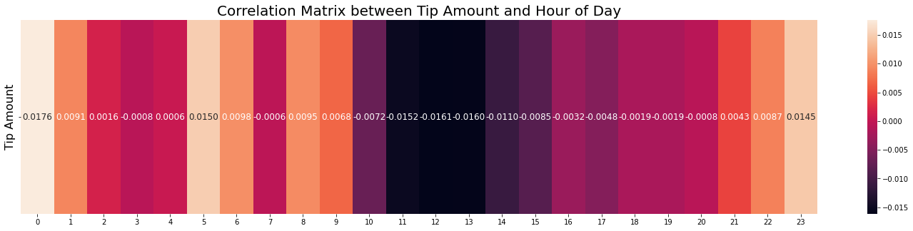
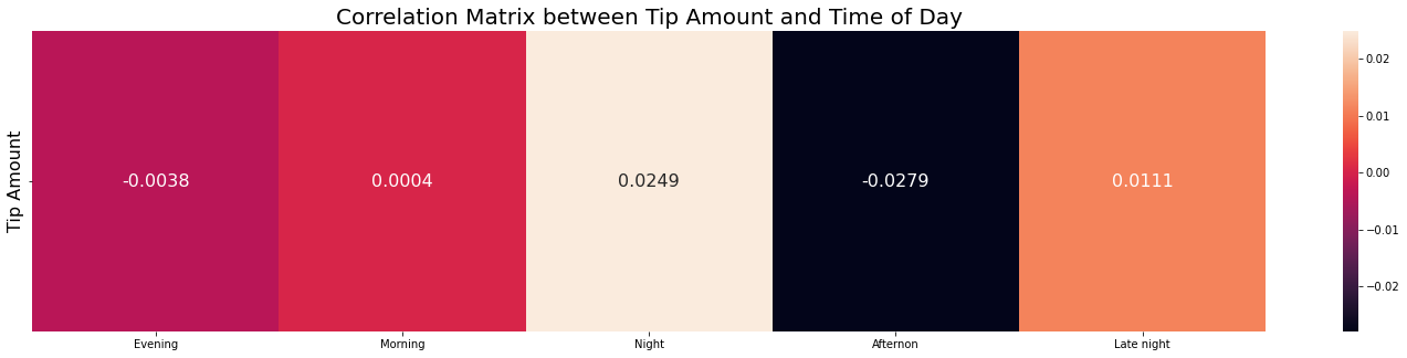
We saw earlier that there isn’t a significant difference between the tipping of various time of the day on average but we can also investigate the correlation as well
columns=list(range(0,24))correlation_hour=pd.DataFrame(index=["tip_amount"],columns=columns)hour_one_hot=pd.get_dummies(df_train.dropoff_hour)fori,colinenumerate(columns):cor=df_train.tip_amount.corr(hour_one_hot[col])correlation_hour.loc[:,columns[i]]=corplt.figure(figsize=(25,5))g=sns.heatmap(correlation_hour,annot=True,fmt='.4f',annot_kws={"fontsize":12})g.set_yticklabels(['Tip Amount'],fontsize=16)plt.title("Correlation Matrix between Tip Amount and Hour of Day",fontdict={'fontsize':20})plt.plot()columns=df_train.dropoff_time_of_day.unique()correlation_tday=pd.DataFrame(index=["tip_amount"],columns=columns)tday_onehot=pd.get_dummies(df_train.dropoff_time_of_day)fori,colinenumerate(columns):cor=df_train.tip_amount.corr(tday_onehot[col])correlation_tday.loc[:,columns[i]]=corplt.figure(figsize=(25,5))g=sns.heatmap(correlation_tday,annot=True,fmt='.4f',annot_kws={"fontsize":16})g.set_yticklabels(['Tip Amount'],fontsize=16)plt.title("Correlation Matrix between Tip Amount and Time of Day",fontdict={'fontsize':20})plt.plot()
Again no significant correlation, but we can still go even further with simple linear regression
Notes: [1] Standard Errors assume that the covariance matrix of the errors is correctly specified.
1
lr2.summary()
OLS Regression Results
Dep. Variable:
tip_amount
R-squared:
0.001
Model:
OLS
Adj. R-squared:
0.001
Method:
Least Squares
F-statistic:
380.3
Date:
Sun, 30 Oct 2022
Prob (F-statistic):
0.00
Time:
06:35:26
Log-Likelihood:
-2.5454e+06
No. Observations:
1182030
AIC:
5.091e+06
Df Residuals:
1182025
BIC:
5.091e+06
Df Model:
4
Covariance Type:
nonrobust
coef
std err
t
P>|t|
[0.025
0.975]
const
1.4439
0.005
300.591
0.000
1.434
1.453
Afternon
-0.2440
0.007
-36.964
0.000
-0.257
-0.231
Evening
-0.1314
0.006
-22.143
0.000
-0.143
-0.120
Late night
-0.0448
0.008
-5.577
0.000
-0.061
-0.029
Morning
-0.1181
0.006
-19.483
0.000
-0.130
-0.106
Omnibus:
1253963.407
Durbin-Watson:
2.001
Prob(Omnibus):
0.000
Jarque-Bera (JB):
385045385.766
Skew:
4.830
Prob(JB):
0.00
Kurtosis:
90.890
Cond. No.
6.67
Notes: [1] Standard Errors assume that the covariance matrix of the errors is correctly specified.
From this analysis we see that 1AM and 6AM are insignificant while most other hours of the day contribute negatively to the average tipping amount except for 5AM as expected.
We can go even further by trying to model the tipping amount with the features we have. I’ll opt for s Random Forest Model, which I will probably write about in the future along with tree models. The code for this is as follows:
We also cyclically encode the time feature (dropoff hour), this is usually done when we have cyclical features such as hour of the day, days of the week, and others. This can be achieved by taking the sine and cosine of the cyclical feature divided by the period (total number/maximum number of the feature, i,e. 7 if days of the week and 24 if hours). We also one-hot encode our categorical variables. I’ll also write a future article about cyclical encoding of features in the future. We evaluate how well the model performs on our training data.
1
print("Coefficient of determination (R^2) of the model is: ",rf_pipe.score(X,y))
Coefficient of determination (R^2) of the model is:
0.962619575415421
Eventually we would like to see the most important deatures that contribute to predicting the tipping amount (More on this in a future article)
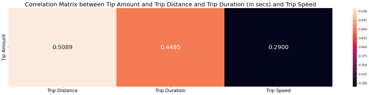
We see that a major influencing factor in determining the tipping amount is how long the trip took and what payment method was used (Cash in our case as intuitively that’s what most people tip taxi rides with). We can see the correlation between the tip, time taken and distance to confirm that there is a correlation but a weak one.
Seeing this we analyze this again with linear regression modelling the average tipping amount
Notes: [1] Standard Errors assume that the covariance matrix of the errors is correctly specified.
1
print(f"On Average {np.round(scaler.inverse_transform(lr_duration.params['x1'].reshape(1,-1))[0][0],0)} seconds or 20 minutes contribute to a 1 dollar tip")
On Average 1249.0 seconds or 20 minutes contribute to a
1 dollar tip
This sums up our findings and this article. I have conducted other analysis as well as a prediction model for predicting the pickup density after clustering New York into several buckets/regions and binning of time. All of this can be found in the projects GitHub repository.
Thank you for reading and if you have any questions regarding the project I’m an email away. Until next time, Bye!