Polynomial Regression

Introduction
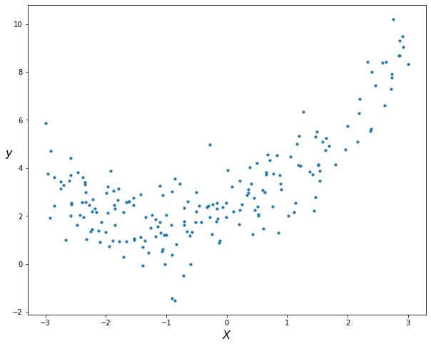
The data we have frequently cannot be fitted linearly, and we must use a higher degree polynomial (such as a quadratic or cubic one) to be able to fit the data. When the relationship between the dependent ($Y$) and the independent ($X$) variables is curvilinear, as seen in the following figure (generated using numpy based on a quadratic equation), we can utilise a polynomial model.
|
|
Understanding linear regression and the mathematics underlying it is necessary for this topic. You can read my previous article on Linear Regression if you aren’t familiar with it.
Applying a linear regression model to this dataset first will allow us to gauge how well it will perform.
|
|
The plot of the best fit line is:
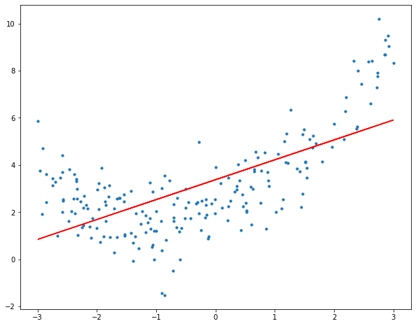
It is clear that the straight line is incapable to depict the data’s patterns. This is an example of underfitting (“Underfitting is a scenario in data science where a data model is unable to capture the relationship between the input and output variables accurately, generating a high error rate.."). Computing the R2 score of the linear line gives:
|
|
R-Squared of the model is 0.42763591651827204
Why Polynomial Regression?
We can add powers of the original features as additional features to create a higher order equation. A linear model,
$\hat{y} = {\alpha} + {\beta}_1x$
can be transformed to
$\hat{y} = {\alpha} + {\beta}_1x + {\beta}_2x^{2}$
What we are only doing here is adding powers of each feature as new features (interactions between multiple features can also be added as well depending on the implementation), then simply train a linear model on this extended set of features. This is the essence of Polynomial Regression (details later 😉)
The scikit-Learn PolynomialFeatures class can be used to transform the original features into their higher order terms. Then we can train a linear model with those new generated features. Numpy also offers a polynomial regression implementation using numpy.polyfit (check my github for usage).
|
|
Fitting a linear regression model on the transformed features gives the following plot.
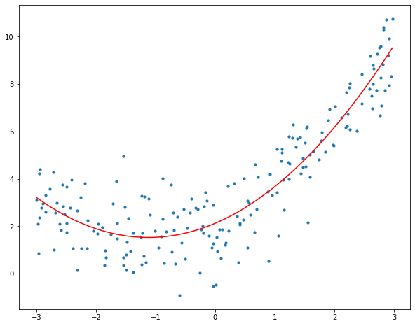
The figure makes it quite evident that the quadratic curve can fit the data more accurately than the linear line. Calculating the quadratic plot’s R2 score results in:
|
|
R-Squared of the model is 0.8242378566950601
Which is a great improvement from the previous R2 score
When we try to fit a curve with degree 10 to the data, we can observe that it “passes through” more data points than the quadratic and linear plots.
|
|
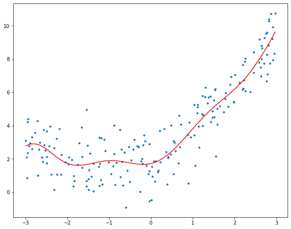
R-Squared of the model is 0.831777739222978
We can observe that increasing the degree to 30 causes the curve to pass through more data points.
|
|
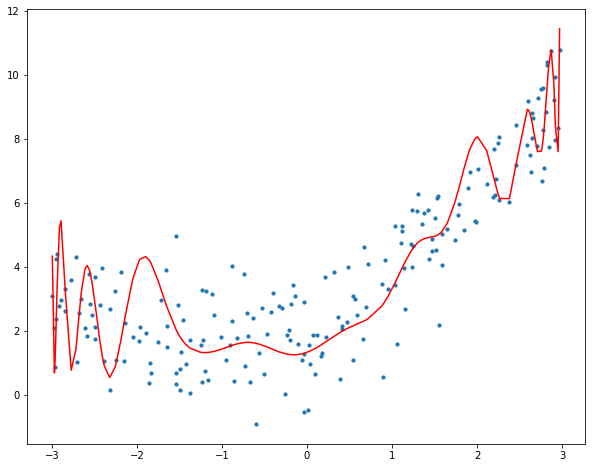
R-Squared of the model is 0.7419383093794893
For degree 30, the model also accounts for noise in the data. This is an example of overfitting ( “Overfitting is a concept in data science, which occurs when a statistical model fits exactly against its training data. When this happens, the algorithm unfortunately cannot perform accurately against unseen data, defeating its purpose.” ). Despite the fact that this model passes through many of the data, it will fail to generalise on unseen data, as observed on the decrease in R2 score.
Before we jump into the details of polynomial regression we must answer an important question, How do we choose an optimal model? And to answer this question we need to understand the bias vs variance trade-off.
The Bias vs Variance Trade-Off
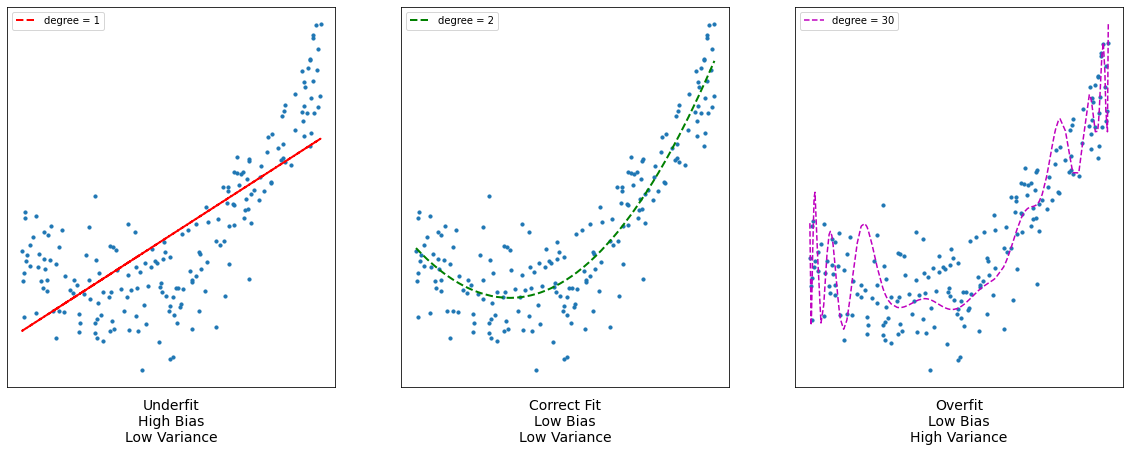
Bias refers to the error due to the model’s simplistic assumptions in fitting the data. A high bias means that the model is unable to capture the patterns in the data and this results in underfitting.
Variance refers to the error due to the complex model trying to fit the data. High variance means the model passes through most of the data points and it results in overfitting the data.
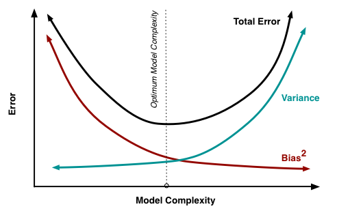
The following figure summarizes this concept:
The graph below shows that as model complexity increases, bias decreases and variance increases, and vice versa. A machine learning model should ideally have low variance and bias. However, it is nearly difficult to have both. As a result, a trade-off is made in order to produce a good model that performs well on both train and unseen data.
Polynomial Fitting Details
Rank of a matrix
Suppose we are given a $mxn$ matrix $A$ with its columns to be $[ a_1, a_2, a_3 ……a_n ]$. The column $a_i$ is called linearly dependent if we can write it as a linear combination of other columns i.e. $a_i = w_1a_1 + w_2a_2 + ……. + w_{i-1}a_{i-1} + w_{i+1}a_{i+1} +….. + w_{n}a_{n}$ where at least one $w_{i}$ is non-zero. Then we define the rank of the matrix as the number of independent columns in that matrix. $Rank(A)$ = number of independent columns in $A$.
However there is another interesting property that the number of linearly independent columns is equal to the number of independent rows in a matrix (proof). Hence $Rank(A) ≤ min(m, n)$. A matrix is called full rank if $Rank(A) = min(m, n)$ and is called rank deficient if $Rank(A) < min(m, n)$.
Pseudo-Inverse of a matrix
An $nxn$ square matrix $A$ has an inverse $A^{-1}$ if and only if $A$ is a full rank matrix. However a rectangular $mxn$ matrix $A$ does not have an inverse. If $A^{T}$ denotes the transpose of matrix $A$ then $A^{T}A$ is a square matrix and Rank of $(A^{T}A)$ = $Rank (A)$ (proof).
Therefore if $A$ is a full-rank matrix then the inverse of $A^{T}A$ exists. And $(A^{T}A)^{-1}A^{T}$ is called the pseudo-inverse of $A$. We’ll see soon why it is called so.
Details
As discussed earlier, in polynomial regression, the original features are converted into polynomial features of required degree $(2,3,..,n)$ and then modeled using a linear model. Suppose we are given $n$ data points $pi = [ x_{i1} ,x_{i2} ,……, x_{im} ]^{T} , 1 ≤ i ≤ n$ , and their corresponding values $vi$. Here $m$ denotes the number of features that we are using in our polynomial model. Our goal is to find a nonlinear function $f$ that minimizes the error
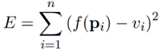
Hence $f$ is nonlinear over $pi$.
So let’s take an example of a quadratic function i.e. with $n$ data points and 2 features. Then the function would be

The objective is to learn the coefficients. Hence we have $n$ points $pi$ and their corresponding values $vi$; we have to minimize
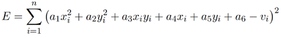
For each data point we can write equations as
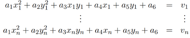
Hence we can form the following matrix equation $$Da = v$$
where
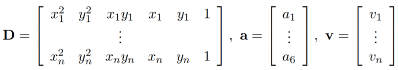
However the equation is nonlinear with respect to the data points $pi$, it is linear with respect to the coefficients $a$. So, we can solve for a using the linear least square method.
We have $$Da = v$$
multiply $D^{T}$ on both sides $$D^{T}Da = D^{T}v$$
Suppose $D$ has a full rank, that is when the columns in $D$ are linearly independent, then $D^{T}D$ has an inverse.Therefore $$(D^{T}D)^{-1}(D^{T}D)a = (D^{T}D)^{-1}D^{T}v$$
We now have $$a = (D^{T}D)^{-1}D^{T}v$$
Comparing it with $Da = v$, we can see that $(D^{T}D)^{-1}D^{T}$ acts like the inverse of $D$. So it is called the pseudo-inverse of $D$.
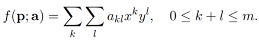
The above used quadratic polynomial function can be generalised to a polynomial function of order or degree $m$.
Thank you for reading and I hope now that you are clear with the working of polynomial regression and the mathematics behind. I have used polynomial regression on the Covid-19 data and wrote an article about it, you can read it here.
Also check the github repo for the complete code.