Confounding Variables in Regression Analysis

Introduction

In today’s article I will be writing about the concept of confounding variables and also include code examples with two datasets as an example. In classical statistics, confounding variable is a critical concept since it can distort our view about input variables and outcome variable’s relationship, while confounding is not a frequent topic that shows up in machine learning and predictive analysis even though it is an important concept that should be understood to fully comprehend regression analysis.

What does confounding mean?

Let’s start by defining what the word confounding means and according to Oxford confounding means to mix up something, which explains the concept well as confounding happens when the effect of our variable of interest is stuck together or mixed with or confounded with another variable. Basically a confounding variable is a type of extraneous variable that is related to both the independent and dependent variables and it must meet two conditions to be a confounder which are:

• It must be correlated with the independent variable. This may be a causal relationship, but it does not have to be.
• It must be causally related to the dependent variable

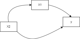
So let’s say we have our dependent variable $y$ and two other independent variables $X_1$ and $X_2$, with the help of a diagram we can further understand confounding.

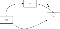
So we’re going to recall when fitting a regression model (check my article on Linear Regression here), we get the equation $y = {\beta}_0 + {\beta}_1X_1$ and that the learned parameter ${\beta}_1$ tells us what effect does $X_1$ have on the outcome ($y$), we update the diagram to indicate where this learned parameter lies:

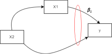
Now there might be some other variable, $X_2$, that’s associated with $X_1$ as portrayed in the diagram, and it can be distorting the effect of $X_1$ on $y$ because these two effects can be stuck together. So the effect that $X_1$ has on y and the effect that $X_2$ has on y are a little bit stuck together as shown here:

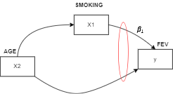
And this happens when $X_2$ is not included in the model. So let’s just think of this example dataset (we’ll explore it later). We have an age variable, we have a smoking variable, and we have the FEV or forced expiratory volume which measures how much air a person can exhale during a forced breath (in other words a persons lung capacity). Both the age and smoking variables are our independent variables and the FEV will be our dependent variable we are trying to predict, portrayed in the diagram as such:

And our goal here is to try and estimate what effect the smoking has on the lung capacity of these people. Now let’s suppose that age is not included in the model. And lets say we discovered from analyzing this dataset is that these smokers are older on average than the non-smokers. This data set is kids ranging from 3 to 19 years old. So the 3, 4, 5, 6, 7, 8, etc. years olds are non-smokers. So the non-smokers on average are younger. And what do we know about this? Younger kids have smaller bodies i.e. smaller lung capacities. Older kids have bigger bodies, bigger lung capacities. The smokers are older on average. So the effect of smoking and the effect of age are going to be a bit stuck together if we don’t include age in the model. When we include age in the model then the equation of the model changes to $y = {\beta}_0 + {\beta}_1X_1 + {\beta}_2X_2$. Then the coefficient/parameter ${\beta}_1$, gives us what’s the effect of smoking on FEV adjusting for the age. So we’re comparing the smoking effect for two people who are the same age. With this in mind we can ask ourselves how can confounding occur?

How does confounding occur?

The way confounding can occur (in the example given; applicable to any regression model) is if the age variable ($X_2$) distribution is different for smoking and non-smoking ($X_1$). But how can we identify that is actually occurred?

Identifying confounding

Some of the ways in identifying confounding are:

• $X_2$ and $X_1$ are associated (some association between the variables)
• $X_2$ is also associated with the outcome ($y$)
• $X_2$ is on the “pathway” between $X_1$ and $y$, what is meant by that is that $X_1$ has a direct effect on $X_2$ which then has an effect on the outcome $y$ shown here:

this is called mediation and $X_2$ in this case is a mediator. And we’re saying that confounding can occur when $X_1$ directly effects $X_2$ WHICH THEN effects the outcome $y$.

• It makes sense conceptually. What is meant by this is that we don’t want to just see that numerically (possibly via correlation) our variables ($X_1$ and $X_2$) are associated but that the association should make sense conceptually. Does it make sense that the age distribution of smokers and non-smokers would be different? And I’d say yes, I think it does. If we’re looking at a group of kids as they get older, they’re more likely to smoke. Doesn’t mean they’re going to, but that association makes sense. And for the second point. Does it make sense that age has an effect on lung capacity? Yes, it does. As kids get older, their bodies get bigger and their lungs should get bigger as well.
• When we adjust for $X_2$ (including it in the model), the parameter ${\beta}_1$ changes significantly, there is no rule for how much it should change but the idea is that it shouldn’t stay the same and it should change a decent amount (if there wasn’t confounding it will most probably stay the same because most of the loss functions used to estimate the coefficients have a global minimum and are convex, so there is only one solution to the regression estimation problem). This tells us that some of the $X_2$ effect was mixed in to the $X_1$ effect.

Residual Confounding

Residual confounding is the bias/distortion that is still left over even after we adjust for the variable (age in our case, $X_2$). This often happens when binning (categorizing) our variable, for example say instead of the actual age we have a categorical variable, age category/group that is in ranges such as 0-4, 5-10, 11-20, etc. Including this variable in the model will help in adjusting for age a bit but it’s not going to be a very good adjustment there is still going to be some confounding (age confounding) left over even after we have adjusted for age in some way.

Confounding and Predictive Accuracy

During my learning journey I ran into this “problem” a couple of times so it is extremely important to understand and have a good grasp on the topic to be able to efficiently deal with it whenever it arises.

You see in the previous paragraph I put the word problem between two quotation marks, this is because confounding is usually regarded as a negative effect and as it should be but at the same time it can also assist the analyst in understanding the data and the variables more, it depends from what angle you’d like to see the problem, nevertheless objectively for measuring effect sizes it is an issue. I mention here effect sizes not predictive accuracy as confounding only affects effect sizes and not predictions. Confounding is less of an issue while making prediction since we are not interested in determining the exact effect of one variable on another. We just want to know what the most probable value of a dependent variable is given a collection of predictors. So for example, suppose that we would like to estimate to what degree a person’s age effects their salary. So we can estimate the model: $salary_i={\beta}_0+{\beta}_1age_i$. It is very likely that ${\beta}_1$ in the equation above will be positive and fairly large, because older people tend to have more education and more work experience. So if we wish pin-point the link between age and salary (effect size), we should probably control for these confounders, estimating the model: $${\beta}_0+{\beta^*}_1age_i+{\beta}_2education_i+{\beta}_3experience_i$$

It is very likely that $${\beta}^* < {\beta}_1$$ and that ${\beta}^*$ will be a much better estimator for the pure effect of age on one’s earnings. That, in the sense of “change someone’s age and keep EVERYTHING else fixed”. However, since age is highly correlated with education and experience, the first model might just be good enough for predicting a person’s salary

Note: Confounding is a problem for prediction when the confounding relationship changes. This is a common problem for ML models in production. E.g., see What We Can Learn From the Epic Failure of Google Flu Trends

Example on King County Housing Data

The data can be found in King County’s official public data website here, data was downloaded from 2014-15. We’ll start first by applying a linear regression model to predict the house price using these predictors/features: AdjSalePrice, SqFtTotLiving, SqFtLot, Bathrooms, Bedrooms, BldgGrade. All code can be found here

 1
 2
 3
 4
 5
 6
 7
 8
 9
10

import pandas as pd
import numpy as np
import matplotlib.pyplot as plt
from sklearn.metrics import r2_score, mean_squared_error
from sklearn.linear_model import LinearRegression

data = pd.read_csv("data/king_county.csv", sep="\t")
predictors = ['AdjSalePrice', 'SqFtTotLiving', 'SqFtLot', 'Bathrooms', 'Bedrooms', 'BldgGrade']
outcome = 'AdjSalePrice'
data[predictors].head()

1
2
3
4
5
6
7

model = LinearRegression()
model.fit(data[predictors], data[outcome])

print(f'Intercept: {model.intercept_:.3f}')
print('Coefficients:')
for name, coef in zip(predictors, model.coef_):
    print(f' {name}: {coef}')

Intercept: -521871.368
Coefficients:
SqFtTotLiving: 228.8306036024076
SqFtLot: -0.06046682065307258
Bathrooms: -19442.840398320994
Bedrooms: -47769.955185214334
BldgGrade: 106106.96307898096

The issue with confounding variables is one of omission: a key variable is missing from the regression equation. An improper interpretation of the equation coefficients might result in incorrect findings. Taking for example our dataset and model, the regression coefficients of SqFtLot, Bathrooms, and Bedrooms are all negative (unintuitive). The regression model does not contain a variable to represent location which is a very important predictor of house price. To model location, I’ll include a variable zip group that categorizes the zip code into one of five groups, from least expensive (0) to most expensive (4) (There are 80 zip codes in King County, several with just a handful of sales. An alternative to directly using zip code as a categorical variable, zip group clusters similar zip codes into a single group).

 1
 2
 3
 4
 5
 6
 7
 8
 9
10
11
12
13
14
15
16
17

zip_groups = pd.DataFrame([
    *pd.DataFrame({
        'ZipCode': data['ZipCode'],
        'residual' : data[outcome] - model.predict(data[predictors]),
    })
    .groupby(['ZipCode'])
    .apply(lambda x: {
        'ZipCode': x.iloc[0,0],
        'count': len(x),
        'median_residual': x.residual.median()
    })
]).sort_values('median_residual')
zip_groups['cum_count'] = np.cumsum(zip_groups['count'])
zip_groups['ZipGroup'] = pd.qcut(zip_groups['cum_count'], 5, labels=False, retbins=False)
to_join = zip_groups[['ZipCode', 'ZipGroup']].set_index('ZipCode')
data = data.join(to_join, on='ZipCode')
data['ZipGroup'] = data['ZipGroup'].astype('category')

We have added this new grouping feature to our dataset

1
2
3
4
5
6
7
8
9

new_predictors = ['SqFtTotLiving', 'SqFtLot', 'Bathrooms', 'Bedrooms', 'BldgGrade', 'PropertyType', 'ZipGroup']
outcome = 'AdjSalePrice'
X = pd.get_dummies(data[new_predictors], drop_first=True)
confounding_model = LinearRegression()
confounding_model.fit(X, data[outcome])
print(f'Intercept: {confounding_model.intercept_:.3f}')
print('Coefficients:')
for name, coef in zip(X.columns, confounding_model.coef_):
    print(f' {name}: {coef}')

Intercept: -666637.469
Coefficients:
SqFtTotLiving: 210.61266005580183
SqFtLot: 0.4549871385465901
Bathrooms: 5928.425640001864
Bedrooms: -41682.871840744745
BldgGrade: 98541.18352725943
PropertyType_Single Family: 19323.625287919334
PropertyType_Townhouse: -78198.72092762386
ZipGroup_1: 53317.173306597986
ZipGroup_2: 116251.58883563547
ZipGroup_3: 178360.53178793367
ZipGroup_4: 338408.60185652017

ZipGroup 0 is not there as we did drop_first = True.

ZipGroup is certainly a key variable: a house in the most expensive zip code group is expected to sell for a higher sales price by almost 340,000 dollars. The SqFtLot and Bathrooms coefficients are now positive, and adding a bathroom raises the sale price by 5,928 dollars. Bedrooms’ coefficient is still negative. While this may appear odd, it is a well-known phenomena in real estate. Having more and hence smaller bedrooms is connected with less value houses for homes of the same living size and number of bathrooms.

Checking Confounding with Lung Capacity Dataset

The data can be found in Kaggle here.

We’ll use ths dataset to check and see if age seems to be confounding the effect of smoking on FEV (lung capacity). The first thing we can do is check if the age distribution is similar or different for smokers or non-smokers, in other words is there an association between age and smoking. To visually examine this we can look at a boxplot which is usually a good way to check for association between different groups and a numerical variable.

1
2
3
4
5

lung = pd.read_csv("data/lung.txt", sep="\t")
import plotly.express as px
fig = px.box(lung, x="Smoke", y="Age")
fig.show()

And here we can see that the smokers are much older on average than the non-smokers so there does appear an association. If we think about it, what direction would the association go in? Does age affect smoking? Or does smoking affect age? Well of course age is going to affect smoking and not the opposite and does this association make sense conceptually aside from being numerically present in the data? Sure it does, as explained above as kids get older they are more likely to become a smoker.

Now we can check if age is associated with FEV, to visually explore this we can plot a scatter plot (two numerical variables).

1
2

fig = px.scatter(lung, x= "Age", y= "LungCap", labels={"LungCap": "FEV"})
fig.show()

We can see a pretty strong association here, we can also quantify that numerically:

1

lung.Age.corr(lung.LungCap)

0.8196748974989415

Again a pretty strong association/correlation. And what would the direction of this association, well lung capacity can’t have an effect on your age and it’s going to be that age that has an effect on lung capacity, getting older means the lung capacity gets larger. Does this association make sense conceptually? Again yes it does.

Now let’s fit a linear regression model that includes age so we can adjust for it statistically:

1
2
3
4
5
6

import statsmodels.api as sm #Use statsmodels for R style summary
vars = ['Age', 'Smoke']
X= pd.get_dummies(lung[vars], drop_first=True)
model_adj = sm.OLS(lung['LungCap'], X.assign(const=1))
res = model_adj.fit()
res.summary()

The coefficient for smoking is now -0.6486, so the interpretation for this would be that for someone who smokes we would expect the mean FEV to be 0.65 litres lower than a non-smoker when we adjust for age. Another way to phrase this is if we take two people who are the same age, on average we’d expect the smoker’s lung capacity to be 0.65 liters lower than the non-smoker. This is what we mean by statistically adjusting for age or statistically adjusting for this confounder.

I also fitted a linear regression model without the age variable and got a coefficient of 0.87 for the smoking variable which shows the negative effect of confounding in interpreting the model coefficients and effect sizes (even though we get the same predictions).

Multicollinearity is another closely related topic to confounding that I will also write about in the future. For now this is it.

Thank you for reading and until next time.